 |
URBAN FOOTPRINT OF MUMBAI - THE COMMERCIAL CAPITAL OF INDIA |
 |
|
Ramachandra. T.V 1,2,3,*, Bharath H. Aithal2, Sowmyashree M.V1 |
| Citation: Ramachandra T. V., Bharath H. A. and Sowmyashree M. V., 2014. Urban footprint of Mumbai - the commercial capital of India, Journal of Urban and Regional Analysis, VI (1): 71– 94 |
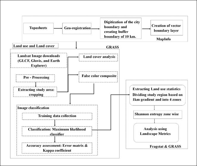
Methods Urban dynamics was assessed using temporal remote sensing data of the period 1973 to 2010. The time series spatial data acquired from Landsat Series Multispectral sensor (57.5m) and thematic mapper (28.5m) sensors for the period 1973 to 2010 were downloaded from a public domain (http://glcf.umiacs.umd.edu/data; http://www.glovis.usgs.gov; http://www.landcover.org/). Survey of India (SOI) topographic sheets of 1:50000 and 1:250000 scales were used to generate base layers of city boundary, etc. The process of the analysis is threefold as described in Figure 3, which includes pre-processing, analysis of land cover and land use, and finally, the gradient wise zonal analysis of Mumbai.
4.1 Pre-processing: Remote sensing data (Landsat series) for Mumbai, acquired for different time periods, were downloaded from Global Land Cover Facility (http://www.glcf.umd.edu/index.shtml) and (http://www.landcover.org/), United States Geological Survey (USGS) Earth Explorer (http://edcsns17.cr.usgs.gov/NewEarthExplorer/) and Glovis (http://www.glovis.usgs.gov). The remote sensing data obtained were geo-referenced, geo-corrected, rectified and cropped pertaining to the study area. Geo-registration of remote sensing data (Landsat data) has been done using ground control points collected from the field using pre calibrated GPS (Global Positioning System) and also from known points (such as road intersections, etc.) collected from geo-referenced topographic maps published by the Survey of India. The Landsat satellite data of 1973 (with spatial resolution of 57.5 m x 57.5 m (nominal resolution) and 1992 - 2009 (28.5 m x 28.5 m (nominal resolution)) were resampled to 30 m in order to maintain uniformity in spatial resolution across different time periods. The study has been carried out for the Mumbai administrative area with 10 km buffer, which helps in accounting the region experiencing sprawl. 4.2 Land Cover analysis: Land Cover analysis was performed to understand the changes in the vegetation cover. Normalised Difference Vegetation Index (NDVI) was found suitable and was used for measuring vegetation cover. NDVI values range from -1 to +1. Very low values of NDVI (-0.1 and below) correspond to soil or barren areas of rock, sand, or urban built up. Zero indicates water cover. Moderate values represent low density vegetation (0.1 to 0.3), while high values indicate thick canopied vegetation (0.6 to 0.8). 4.3 Land use analysis: The method involves i) generation of False Colour Composite (FCC) of remote sensing data (bands – green, red and NIR). This helped in locating heterogeneous patches in the landscape ii) selection of training polygons (these correspond to heterogeneous patches in FCC) covering 15% of the study area and uniformly distributed over the entire study area, iii) loading these training polygons co-ordinates into pre-calibrated GPS, iv) collection of the corresponding attribute data (land use types) for these polygons from the field. GPS helped in locating respective training polygons in the field, v) supplementing this information with Google Earth, vi) 60% of the training data has been used for classification, while the balance is used for validation or accuracy assessment. Land use analysis was carried out using supervised pattern classifier - Gaussian Maximum Likelihood Classifier (GMLC) algorithm. Remote sensing data was classified using signatures from training sites that include all the land use types detailed in table 3. Mean and covariance matrix are computed using estimate of maximum likelihood estimator. This technique has proved to be a superior classifier as it uses various classification decisions using probability and cost functions (Duda et al., 2000, Ramachandra et al., 2012).
Table 3: Land use classification categories adopted Maximum likelihood classifier is then used to classify the data using these signatures generated. This method is considered as one of the superior methods as it uses various classification decisions using probability and cost functions (Duda et al., 2000). Mean and covariance matrix were computed using estimate of maximum likelihood estimator. Land use was computed using the temporal data through the open source program GRASS - Geographic Resource Analysis Support System (http://ces.iisc.ac.in/foss). Signatures were collected from field visits and with the help of Google Earth. 60% of the total generated signatures were used in classification, 40% signatures were used in validation and accuracy assessment. Classes of the resulting image were re-classed and recoded to form four land-use classes Accuracy assessment methods evaluate the performance of classifiers (Mitrakis et al., 2008). This is done either through comparison of Kappa coefficients (Congalton et al., 1983). For the purpose of accuracy assessment, a confusion matrix was calculated. Accuracy assessment and Kappa coefficient are common measurements used in various publications to demonstrate the effectiveness of the classifications (Congalton, 1991; Lillesand & Kiefer, 2005; Bharath H A and Ramchandra, 2012). Recent remote sensing data (2010) was classified using the collected training samples. Statistical assessment of classifier performance based on the performance of spectral classification considering reference pixels is done which include computation of kappa (κ) statistics and overall (producer's and user's) accuracies. For earlier time data, training polygon along with attribute details were compiled from the previously published topographic maps, vegetation maps, revenue maps, etc. 4.4 Zonal Analysis: City boundary along with the buffer region was divided into 4 zones: Northeast (NE), Southwest (SW), Northwest (NW), Southeast (SE) for further analysis as the urbanization is not uniform in all directions. As most of the definitions of a city or its growth are defined in terms of directions, it was considered more appropriate to divide the region in four zones based on direction. Zones were further divided into concentric circles of 1 km incremental radius from the central pixel (Central Business district). The growth of the urban areas along with the agents of changes is understood in each zone separately through the computation of urban density for different periods. 4.5 Division of these zones to concentric circles (Gradient Analysis): All of the zones were divided into concentric circles with a consecutive incrementing radius of 1 km from the center of the city (Ramachandra et al., 2013a). This analysis helped in visualising the process of change at a local level and to understand the agents responsible for the changes. This helps in identifying the causal factors and locations experiencing various levels (sprawl, compact growth, etc.) of urbanization in response to the economic, social and political forces. This approach (zones, concentric circles) also helps in visualizing the forms of urban sprawl (low density, ribbon, leaf-frog development). The built up density in each circle is monitored overtime using time series analysis. This helps the city administration in understanding the urbanization dynamics to provide appropriate infrastructure and basic amenities. 4.6 Shannon’s Entropy: Further to understand the growth of the urban area in a specific zone and to understand if the urban area is compact or divergent, the Shannon’s entropy (Sudhira et al., 2004; Ramachandra et al., 2013b) was computed for each zone. Shannon’s entropy (Hn), given in equation 1, explains clearly the development process and its characteristics. Where Pi is the proportion of the built-up in the ith concentric circle. As per Shannon’s Entropy, if the distribution is maximally concentrated in one circle, the lowest value zero will be obtained. If distribution evenly among the concentric circles, Hn will have maximum of log n. 4.7 Computation of spatial metrics: Spatial metrics are helpful to quantify spatial characteristics of the landscape. Selected spatial metrics were used to analyse and understand the urban dynamics, FRAGSTATS (McGarigal and Marks, 1995) was used to compute metrics at three levels: patch level, class level and landscape level. Table 4 below gives the list of the metrics along with their description considered for the study. Table 4: Spatial metrics chosen for the urban pattern analysis
|
| * Corresponding Author : | |||
| Dr. T.V. Ramachandra Energy & Wetlands Research Group, Centre for Ecological Sciences, Indian Institute of Science, Bangalore – 560 012, INDIA. |
Tel : 91-80-23600985 / 22932506 / 22933099, Fax : 91-80-23601428 / 23600085 / 23600683 [CES-TVR] E-mail : cestvr@ces.iisc.ac.in, energy@ces.iisc.ac.in, Web : http://wgbis.ces.iisc.ac.in/energy |
||