MATERIALS AND METHOD

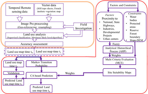
Figure 2 outlines the procedure followed in the quantification and visualization of land use changes. This involved analysis of temporal land uses and visualization of likely changes through consideration of influencing agents.

3.1 Landscape dynamics
The temporal remote sensing data of Landsat ETM+ series (2004, 2007, 2013) were downloaded from GCLF (http://http://glcfapp.glcf.umd.edu:8080/esdi/) and IRS P6 (2010) data was procured from National Remote Sensing Center (http://nrsc.gov.in), India. ASTER DEM (30 m) was used to derive slope details of the region. The Survey of India topographic maps of 1:50000 and 1:250000 scale and online spatial data (http://bhuvan.nrsc.gov.in; https://www.google.com/earth/) were used to generate base layers of administrative boundaries, drainage network, road network, etc. GCPs (Ground control points) and training data is collected using pre calibrated GPS (Global Positioning System) from field.  Land use analyses involved (i) generation of False Color Composite  (FCC)  of  remote  sensing  data  (bands–green,  red  and  NIR), (ii) selection of training polygons (training data) covering 15 % of the study area (polygons are uniformly distributed  over  the  entire  study  area) (iii)  loading  these  training polygons  co-ordinates  into  pre-calibrated  GPS, collection  of  the corresponding attribute data (land use types) for these polygons from  the  field, (iv) supplementing this information with Google Earth and  (v)  60 %  of  the  training  data  has  been  used  for  classification, while  the  balance  is  used  for  validation  or  accuracy  assessment. Error matrix (also referred as confusion matrix) kappa (κ) statistics and overall (producer's and user's) accuracies were assessed. The land use analysis was done using supervised classification technique based on Gaussian maximum likelihood algorithm using remote sensing data and training data collected from field. GRASS GIS (Geographical Resources Analysis Support System, http://ces.iisc.ernet.in/grass), a free and open source software with the robust support for processing both vector and raster data has been used for analyzing RS data.

3.2 Visualisation of forest transitions: Simulation and prediction
Raster maps of the constraining factors and transition factors were generated at common resolution of 30 m for effective processing time. Likely land uses in 2022 is generated by  (i) Markov Chain transition of base land uses, (ii) evaluating the driving factors and constraints, (iii) weightage metric score by fuzzy AHP based estimation and site suitability maps generation by MCE, and (iv) simulation and future prediction of land use by MC-CA algorithms. The transition probability is computed through MC analysis using land use maps of 2004, 2007 and 2010. The driving forces of land use changes and constraints (Table 1 & 2) were identified based on the land use history, review of published literatures and policy reports. Major drivers of landscape transitions are slopes, major highways, industries, core residential areas, etc. Entities such as water bodies, river coarse, protected areas and reserve forest are considered as constraints as they are likely to change. The contributing factors for different land uses were normalized between 0 and 255 through fuzzification, 255 indicates maximum probability of change, while 0 indicates of no changes (Figure 3), which allows to translate qualitative assessment into quantitative data by providing more logical and precise results. Constraints of land use transition is given in Figure 4. The pair wise comparison matrices were generated across three agro climatic regions and their relative weights as Eigen vectors were estimated using AHP [46] to measure the degree of importance between criteria or factors i and j. A response matrix A= [aij] is generated to measure the relative dominance of item i over item j with the decision maker’s assessments aij, as pairwise comparisons that follow a uniform probability distribution (eq 1).

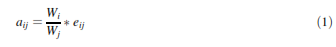
Where, Wi and Wj are the priority weights belongs to vector W and = 1,  is inconsistency observed in the analysis.

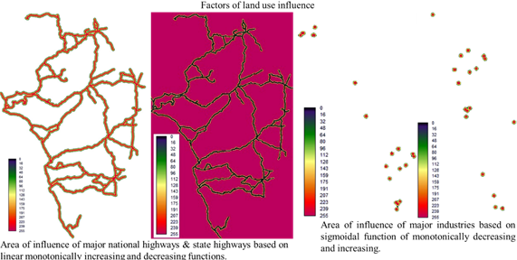
Fig. 3 Factors of land use influence by fuzzy distance tool measurement

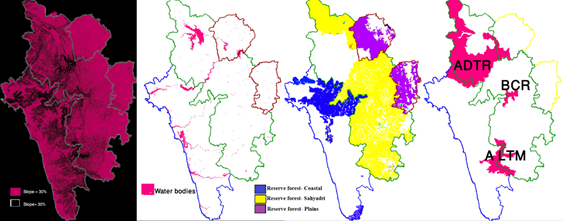
Fig. 4 Constraints of land use transition

The comparison matrix elements were compared pair wise to relate single element at the level directly and ranked by eigenvector of the matrix [47] and eigenvalue of is computed [48]. The consistency index CI is computed to evaluate consistency of the judgment matrix (Eq. 2).  Consistency ratio (CR) were evaluated for three regions and acceptable CR from 0.04 to 0.09 is obtained for each land use (Table 3) based on (Eq. 3). CR value below 0.1 indicates the model is consistent, obtained by the probability of the random weights from the landscape factors [49] and applied for subsequent processes. CA process is implemented based on the site suitability (the probability of that cell’s changing to a given class in the future) and the transition matrix (contains the number of cells that change in the time step derived from the number of cells of each class by multiplying the probability matrix) generated from Fuzzy-AHP. The simulation and prediction of land use changes at every single time step is computed based on current land use and the state of neighboring pixels. Diamond filter of 5 × 5 kernel size was applied to the cellular automata to considered neighborhood land use effects. Two scenarios were designed to emphasize the environmental protection and violation in the region to visualize future state of forests (i) high protection scenario considering the protection of reserve forest with appropriate regulatory mechanism and (ii) least protection scenario (WRF-without reserve forest protection) with increase in population and erosion of forest resources. The Kappa statistic is an excellent measure for comparing a map of “reality” versus some “alternative “map of higher accuracy [50]. The accuracy of prediction is assessed through Kappa statistics by measuring agreement between predicted and actual land uses.

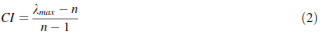
Where, CI is the consistency index, is the largest or principal eigenvalue; n is the order of the matrix. If CI = 0, the matrix had a complete consistency. The worse consistency will represent greater value of CI.
The consistency ratio (CR) is calculated (equation 3) by

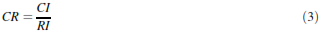
Where, RI is the average of the resulting consistency index depending on order of the matrix. If CR value is less than 0.10, the matrix had a reasonable consistency, otherwise the matrix should be altered for better CR.

Table 1. Driving forces of landscape transition and constraints

Table 2. Constraints of land use change

Table 3. Weightage Eigen vector and consistency ratio of each land use