3.1 Modeling performance and output
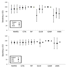
Ensemble modeling approach has shown good performance in our study. MARS, CTA, RF and GAM showed consistently better value for specificity (0.75-1.0) in comparison to GLM and ANN (0.4-0.9) (i.e. AUC, TSS and kappa values), whereas, there is not much difference in sensitivity (Fig 3). Similarly, selection of multiple sets of pseudo-absence points for different sets of algorithms notably improved model performance (Fig 4) although absence point selection strategy has not shown much difference. The role of variables depends on the chosen algorithm and the results indicate that bioclim 7 (annual temperature range), bioclim 10 (mean temperature for warmest quarter), bioclim 16 (precipitation of wettest quarter) and soil moisture played a pivotal role in the model.    

3.    4.      
Figure 3. Modelling performance in terms of sensitivity and specificity (BIOMOD2)

Figure 4. Performance of pseudoabsence points in modeling experiment in BIOMOD2 (a= sensitivity, b=specificity; 1=MARS, 2=CTA, 3=RF, 4=GLM, 5=GAM and 6=ANN)

MaxEnt has shown a better output in comparison to some of the BIOMOD2 based algorithms.  AUC values for training and test data were ≥ 0.95. Similar to BIOMOD2 soil moisture, bioclim 16 (precipitation of wettest quarter), bioclim 10 (mean temperature for warmest quarter) and bioclim 11 (mean temperature of coldest quarter) have shown significant role in the model (Table 1).
The usual approach of getting a final ensembled map has not been followed here due to methodological differences (eg. 3 different sets of pseudoabsense points, 2 different selection strategies etc.) applied in BIOMOD2. The result obtained from each set (i.e. 3 from BIOMOD2 + 1 from MaxEnt = total 4 outputs) has been presented for comparative assessment.

Table 1. Importance of variables in model development (highest contributor under each model is in bold format)

Potential distribution maps generated from these modelling exercises have shown diverse areas ranging from 5,000 – 79,000 km2 (Fig 5 and Table 2).  Both MARS and MaxEnt results have projected near realistic distribution pattern (26,689 and 55,962 km2 respectively) in contrast to CTA-RF and GLM-GAM-ANN ensemble sets (79,985 and 5,144 km2). 

3.2 Conservation status assessment
Potential distribution area for the species based on the extent of occurrence (EOO) is about ~ 47,700 km2 while, area of occupancy (AOO) done by grid method indicate of 116 km2 as currently occupied area (Table 2).

  Table 2. Results of EOO and AOO measurements based on different methods.