Results and discussion

Land cover analysis: Temporal vegetation cover analysis done through the computation of NDVI. This metric helps to understand the changes in the vegetation cover and ranges from values -1 to +1. Very low values of NDVI (-0.1 and below) correspond to soil or barren areas of rock, sand, or urban built-up. Zero indicates the water cover. Moderate values represent low density vegetation (0.1 to 0.3), while high values indicate thick canopy vegetation (0.6 to 0.8). Table 4 tabulates the NDVI values providing the extent of areas under vegetation versus non-vegetation. Figure 4 depicts the land cover change of the study region during 1977, 1980, 1998 and 2010. Temporal analyses of the land cover indicate of decline in vegetation by about 75.03%, while the area under non vegetation has shown an increase of 121%. Further in order to differentiate the impervious layer of urban settlements and other land uses in the non-vegetation category land use analysis was performed.

     

  

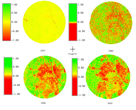
Figure 4: Extent of vegetation assessment through NDVI

Table 4: Land cover (vegetation) based on NDVI

Land use Analysis: Land use analyses for the period 1977 to 2010 have been done through the Gaussian maximum likelihood classifier. Figure 5 depicts the land use during 1977 to 2010. Table 5 lists land use details which indicate that the area under built-up has increased from 3.6 (1977) to 25.06% (2010). Vegetation decreased phenomenally from 41% (in 1973) to 31% (in 2010) with an increase in urban impervious layer. This is significant as this alters the environmental parameters such as ground water recharge, micro-climate, etc. Figure 6 depicts the growth of urban area in the study region in past 4 decades. Accuracy assessment of the classified images was performed by generating the error matrix and kappa statistics. Table 6 depicts the overall accuracy and kappa statistics for the classified images.

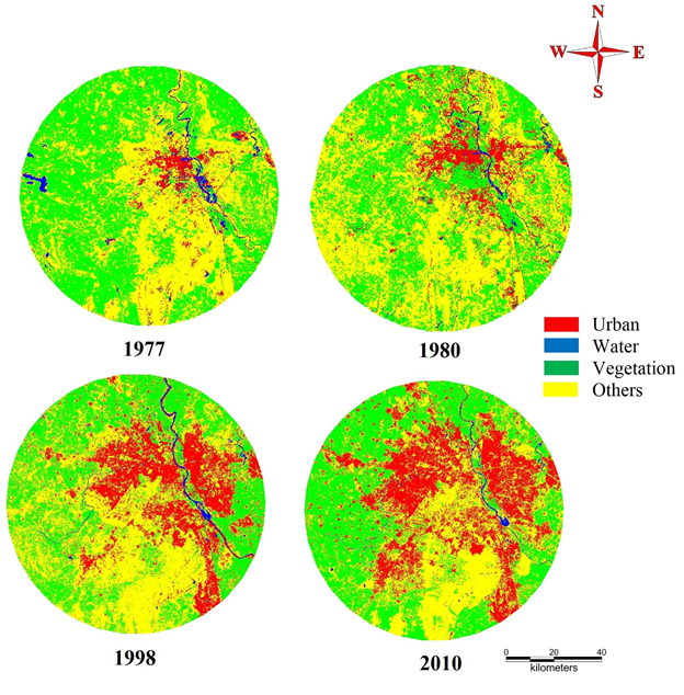
Figure 5: Temporal land use dynamics in Delhi.

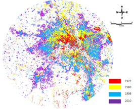
Figure 6: Delhi urbanization process during 1977- 2010

Table 5: Spatial extent of land uses during 1977 to 2010

Table 6: Overall Accuracy and kappa statistics of classified images

Gradient Analysis: The study region was further divided direction-wise into concentric circles and land uses in each sub-region were computed.  Figure 7 illustrates the zone and direction-wise temporal land use changes at local levels. The gradient analysis reveals that North East and North West zones show higher urbanisation trend in 2010 with the economic and industrial dominance.  Agents such as major air bases such as Indira Gandhi International Airport (IGI) and Indian Air force base (Hindon) have contributed to the urban growth in recent years. Delhi Metro which connected core areas radially outskirts also fuelled the growth. This analysis helped in visualizing the zones of urban expansion. Further to charecterise the growth, Shannon entropy was calculated.

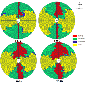
Figure 7: Circle-wise Land Use statistics for Delhi

Shannon’s entropy (Hn): Shannon’s entropy an indicator of growth of urban areas and depicts sprawl rate is computed for all four directions and listed in Table 7. The results indicate that NE and NW regions of the study area are experiencing sprawl. The values of Shannon entropy range from 0 to log (n). Higher the value or closer to log (n) indicates the sprawl or dispersed or sparse development.  Lower the entropy values the development is either aggregated or compact. The results indicated that the city grew phenomenally in the south east and northwest directions during 90’s. Figure 8 depicts that trend urban patches in the northeast and northwest directions are getting fragmented.

Table 7: the Shannon’s entropy to assess the urban sprawl

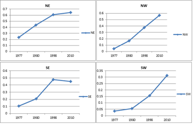
Figure 8: Shannon’s entropy direction-wise for 1977 to 2010

Spatial metrics: Landscape metrics were calculated through Fragstat software using the binary file output from grass.

Percentage of Land (PLAND): PLAND equals the percentage of landscape comprised of the corresponding class patches. Built up percentage was computed to understand the ratio of built up and its increase in the landscape. The analysis shows that percentage of urban landscape is higher in the North-east and South-east direction during 90’s and 2000’s. For North-west direction maximum patch density found majorly to the core areas in circles ranging from C4 to C15. The overall analysis depicts high rate of urbanization in North- east direction during 90’s and in 2010 (Figure 9a).

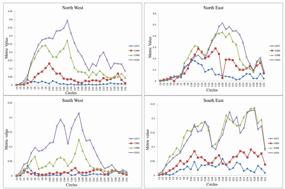
Figure 9a:  the proportion of urban land (PLAND) – circle and zone wise

Number of patches (NP): NP equals the number of built up patches in a landscape. It indicates the level of fragmentation in built up landscape. Figure 9b showed an increasing trend for number of patches from in all directions which also depict that as we move away from the city center the number of patches increases indicating landscape fragmentation. The higher values for year 1990 in all direction, while in 2010 the patches are combining to from a single compact patch. Further it can be seen that the circles in 2010 near the core area of the city in northeast and northwest directions were forming a single dominant patch of urban land use. But South east and south west core regions of the city were fragmented. Number of patches also showed that the Buffer regions of 10kms was highly fragmented in 2010 which has almost least existence of urban land use in 1977.

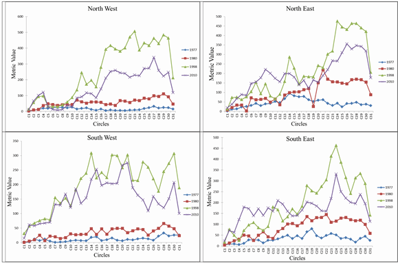
Figure 9b: Number of urban patches

Patch Density: Patch density is an indicator of urban fragmentation. As the number of patches increases, patch density increases which represent higher fragmentation. The patch density also showed the similar trend as the number of patches that is increase in the urban patches in 90’s which indicated the more fragmentation of the urban patches and decreased again for 2000’s. Figure 9c represents that the urban patches were more compact in the core areas and gradually increase as we moves away from the core area which indicate the level of fragmentation in the landscape. Higher patch density during 1990 in all direction indicate of fragmentation and hence the sprawl in the region. Patch density values decreased in 2010 indicating that the smaller patches that had come up were aggregating to form a single large patch. Lower patch density in the core area and the fragmented buffer zones has higher Patch density during 2010 emphasise the intense urbanisation at city center and sprawl at the outskirts.

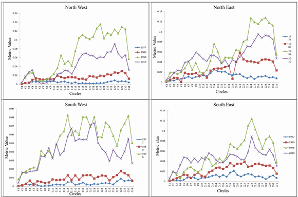
Figure 9c: Urban category patch density

Largest Patch Index (LPI) represents the largest patch and comparative assessment across the years aids in understanding the urbanisation transitions in the region. Figure 9d depicts that largest urban patch in circle C11 and C20 in North-east direction (1990’s). In North-west direction C8 and C15 showed the maximum values for LPI.  In South-east and South-west the largest urban patches were in 2000. This metric helps in identifying the growth poles during different years.

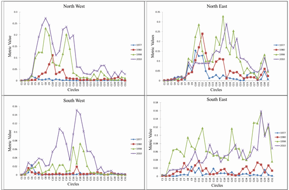
Figure 9d: Largest Patch Index

Area Weighted Mean Shape Index (AWMSI) was computed in which average shape index of patches was weighted by patch areas so that larger patches are weighed higher than smaller ones. It is used to represent shape irregularities, with smaller values indicating more regular shape and as the value increases complexity and irregularities increases. The area-weighted mean shape index (AWMSI) is a robust metric used to describe landscape structure across spatial scales by calculating the complexity of urban patches according to their size (Huang et al., 2009). Figure 9e. Highlight of more compact and regular shapes in the core areas because of which the circles near to core area shows minimum value compared to the circles away from the core area which represent complex and fragmented urban patches.

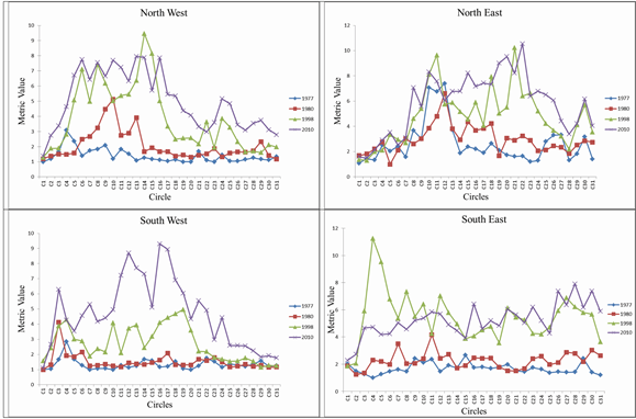
Figure 9e: AWMSI – direction and circle wise

Normalized landscape shape index (NLSI): NLSI provides a simple measure of class through the measure of shape. Figure 9f depicts the results of NLSI. The values close to 0 indicates that the landscape is aggregating to form simple shape, values closer to 1 indicate that landscape is fragmented and has convoluted shapes. Analysis indicates of higher values during 1990 as the landscape started fragmenting, whereas during 2010 the values started decreasing this indicated that each fragment is getting clumped to form a single urban landscape Southeast and southwest directions show maximum variations indicating fragmentation and complexity of urban structure.

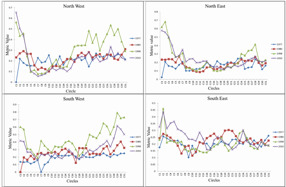
Figure 9f: NLSI of urban landscape

Clumpiness index (CLUMPY): CLUMPY is the measure of urban patch aggregation and ranges from 0 (maximally disaggregated) to 1 (maximally aggregated). Temporal analysis of clumpiness index  for urban category highlights urban dynamics through the process of aggregation of urban patches. Figure 9g with the Clumpy values of  1 at core areas (in 1977) indicates of a clumped growth. The process intensified  during the post globalization era  with  higher CLUMPY values at the city centre and fragmented landscape at outskirts (in 2010).

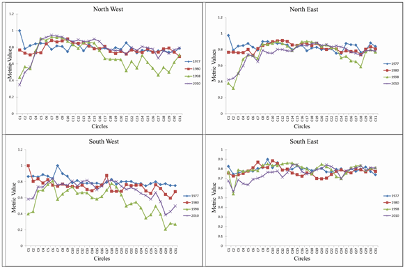
Figure 9g: Clumpiness Index