|
Results and Discussion
pH: The pH of river water is the measure of how acidic or basic the water is on a scale of 0-14. It is a measure of hydrogen ion concentration. Most of the peninsular rivers falls between 6.5 and 8.5 on this scale with 7.0 being neutral. The optimum pH for river water is around 7.4. Water's pH can be altered by industrial and agricultural runoff. Vajgadde at BRB has recorded low pH of 6.9 and Kalghatghi from the same river basic has recorded highest pH of 8.27. In the current study the low range of pH observed in forested streams and high alkaline pH observed in sites contaminated with agricultural and urban runoff (figure 8 and 9). A pH of 8.0 should be sufficient to support most river life with the possible exception of snails, clams, and mussels, which usually prefer a slightly higher pH. The average pH in the study was 6.9, a value that is only sufficiently basic for bacteria, carp, suckers, catfish, and insects. BRB (Bedthi river basin) and KRB (Kali river basin) records most of the alkaline sites, where as ARB (Aghnashini river basin), SRB (Sharavathi river basin) and VRB (Venkatapura river basin) sites records neutral to near acidic sites.
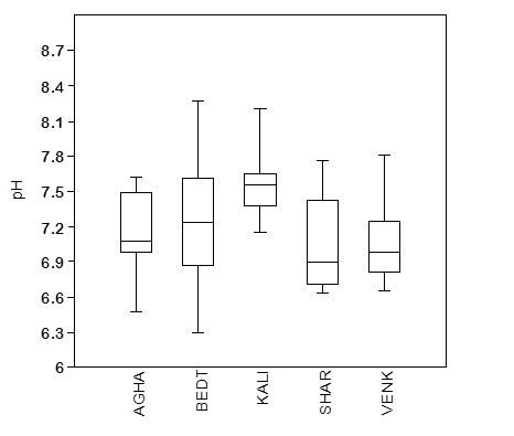
Figure 8: pH across river basins
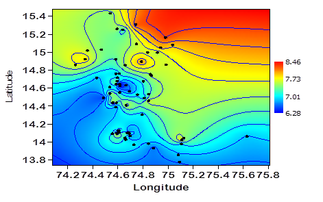
Figure 9: Spatial representation of pH across sites
Electrical Conductivity and Total Dissolved Solids : Conductivity is a measure of the ability of water to pass an electrical current. Conductivity in water is affected by the presence of inorganic dissolved solids such as chloride, nitrate, sulfate, and phosphate anions (ions that carry a negative charge) or sodium, magnesium, calcium, iron, and aluminum cat ions (ions that carry a positive charge). Organic compounds like oil, phenol, alcohol, and sugar do not conduct electrical current very well and therefore have a low conductivity when in water. Conductivity is also affected by temperature: the warmer the water, the higher the conductivity. Low level of electrical conductivity is observed at Vajgadde at BRB (22.5 µS/cm) and highest value was recorded from Kalghatghi of the BRB (1038.95 µS/cm), as illustrated in Figure 10. Sites of BRB showed high levels of variation when compared to the SRB and VRB. KRB sites recorded comparatively high levels of conductivity and total dissolved solids due to sedimentation from the monoculture plantations of its catchment area in the north part of the river basin (Figure 11).
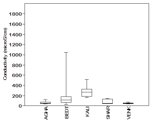
Figure 10: electrical conductivity across river basins
Discharges to streams can change the conductivity depending on their make-up. A failing sewage system would raise the conductivity because of the presence of chloride, phosphate, and nitrate; an oil spill would lower the conductivity.
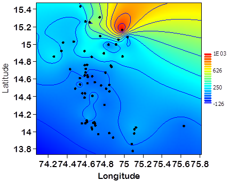
Figure 11: Spatial representation of electrical conductivity across sites
Dissolved Oxygen : An adequate supply of dissolved oxygen gas is essential for the survival of aquatic organisms. A deficiency in this area is a sign of an unhealthy river. There are a variety of factors affecting levels of dissolved oxygen. The atmosphere is a major source of dissolved oxygen in river water. Waves and tumbling water mix atmospheric oxygen with river water. Oxygen is also produced by rooted aquatic plants and algae as a product of photosynthesis.
In the present study lowest dissolved oxygen levels were observed in Kervada (3.67 mg/L) from KRB. This site is located next to the point where the Paper mills effluent confluence with the main river (Figure 12). The paper mill effluent is characterized with high levels of organic content, which consumes most of the oxygen for its degradation with help of the bacteria. Bacteria which decompose plant material and animal waste consume dissolved oxygen, thus decreasing the quantity available to support life. Ironically, it is life in the form of plants and algae that grow uncontrolled due to fertilizer that leads to the masses of decaying plant matter. This site is also infested with marsh crocodiles (Crocodylus palustris), which prevails as a major threat to the humans and cattle in the surrounding s. Crocodiles are attracted to this particular place due to availability of the solid organic contents present the paper mill effluent. Sites at SRB recorded saturated levels of dissolved oxygen in the streams and all other sites recorded with high variation. Apart from the organic pollution other reason for low levels of dissolved oxygen is lack of mixing in water. In most of the middle reaches of all the rivers water is stopped by the small to moderate levels of check dams for agricultural activities. Stagnated water lack gas mixing, which lead to low levels of dissolved oxygen.
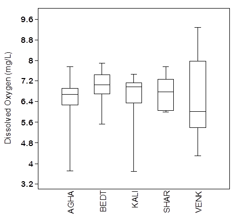
Figure 12: Dissolved Oxygen levels across rive basins
Nutrients: Unlike temperature and dissolved oxygen, the presence of nitrates usually does not have a direct effect on aquatic insects or fish. However, excess levels of nitrates in water can create conditions that make it difficult for aquatic insects or fish to survive. Nitrate-nitrogen is important because it is biologically available and is the most abundant form of nitrogen in Central Western Ghats streams. Like phosphorus, nitrate can stimulate excessive and undesirable levels of algal growth in water bodies. Nitrates come to the streams mainly from the runoff from the agriculture farms and sedimentation. Runoff from the agriculture farms carries huge amount of fertilizer residues. Among the study river basins, KRB (Kali river basin) and BRB (Bedthi river basin) recorded high levels of nitrates from its upstream region (Figure 13). Both KRB and BRB possess intense agriculture and limited water area in its upstream regions which leads to high levels of nitrates.
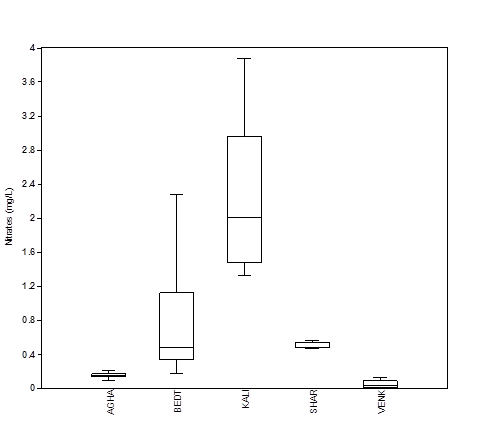
Figure 13: Nitrate across river basins
Along with the nitrates, phosphate also plays an important role in the river hydrobiology. Phosphorus is an important nutrient for plant growth. Total phosphorus is the measure of the total concentration of phosphorus present in a water sample. Excess phosphorus in the river is a concern because it can stimulate the growth of algae. Excessive algae growth, death, and decay can severely deplete the oxygen supply in the river, endangering fish and other forms of aquatic life. Urban runoff is the major source for phosphates in the streams. In the current study regions, BRB receives considerable amount of urban sewage from Hubli city. The impact of high levels of phosphates leads to algal blooms in many reaches of the Bedthi River. Manchikeri site located in between Sirsi and Yellapur have a check dam for pumping water for drinking water supply. Recently a check dam was constructed near the Manchikeri Bridge for storing water for Yellapur drinking water supply. Check dam paves a way to stores the severely polluted water and reduces the dilution of pollution. Stagnated water with heavy nutrient content leads to algal bloom. Preliminary investigations suggest that the algal bloom was created by algal genus Microcystis. Microcystis is a type of blue-green algae (also referred to as Cyanobacteria). This genus is colonial, which means that single cells can join together in groups which tend to float on the water surface. Colony sizes will vary from a few to hundreds of cells. It is a common bloom-forming algae found primarily in nutrient enriched river and lake waters. Any large algal bloom has the potential to result in fish kills by depleting the water of oxygen. The dead algal cells sink down and consume huge amount of oxygen for their decomposition. In such situations, there may not be enough oxygen remaining in the water to support fish in the vicinity. Furthermore, as these large blooms die and sink to the bottom, they commonly release chemicals that can produce a foul odor and musty taste. Some strains of Microcystis may produce toxins that have been reported to result in health problems to animals that drink the water, and minor skin irritation and gastrointestinal discomfort in humans that come in contact with toxic blooms. Uncontrolled growth of single species of algae will also lead to death of aquatic invertebrates and fishes due to unavailability of food, which in turn affects the aquatic food chain.
Lotic Ecosystems: Intra basin variations in quality
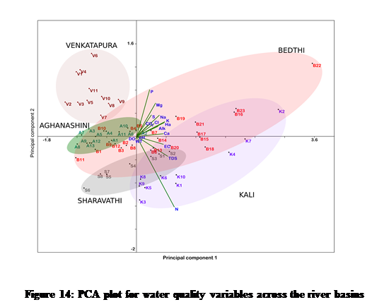
Principal component analysis reveals that BRB (Bedthi River Basin) contains sites with pristine to heavily polluted waters. Most of the sites in BRB in the northern portion stand out separately in ordination space due to their very high amount of ions and nutrients. SRB (sharavathi River Basin), KRB (Kali River Basin) and ARB (Aghanashini River Basin) sites seem to fall in the same quality of water, where as the VRB (Venkatapura River Basin) stands out separately with very pristine water quality status (Figure 14, 15). NMDS plot of the water quality variables shows that ionic and physical parameters have the same origin, where as nutrients arise from different source (Figure 15).
Seasonality of Benthic Diatoms and water quality
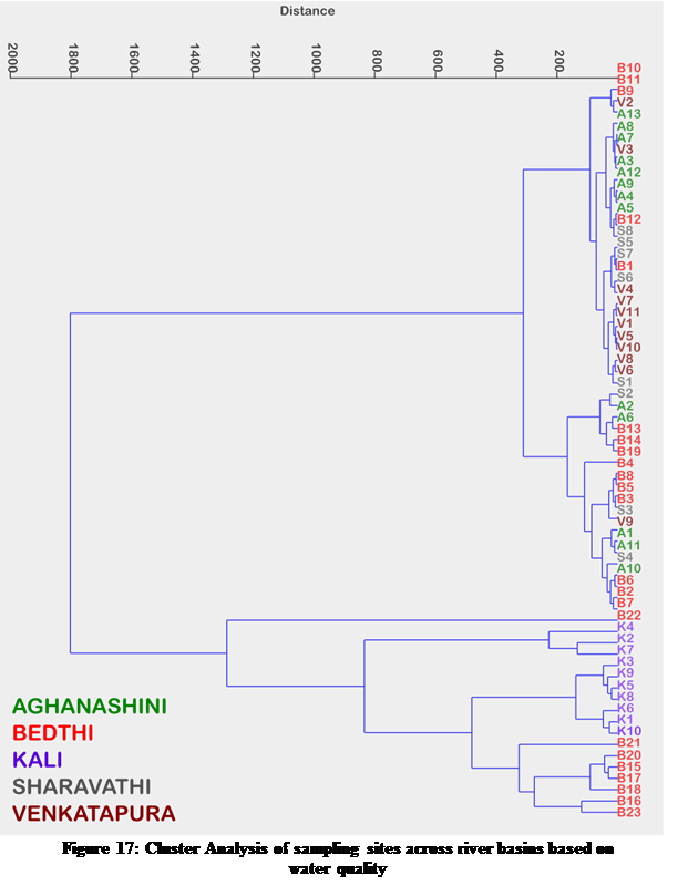
The water chemistry data along the Bedthi River showed high annual variation across sites. The parameters which showed significant different among the groups were pH, conductivity, chlorides, hardness, calcium, magnesium, sodium and potassium. All the above mentioned parameters were high in HPAS, moderate in MPPS and very low in LPFS (Table 3). Irrespective of the pollution status, dissolved oxygen (DO) levels across water quality regimes were roughly similar with mean DO levels (Mean±S.D) of 7.51±1.67, 7.08±2.21, 6.43±2.91. However an anoxic DO level of 0.86 mgL-1 was observed in one sample from the HPAS (KAL). PCA results indicated that water quality differed markedly among sampling sites and across seasons (Figure 14) with the first component explaining 84.6% of the total variation. Three distinct clusters were observed along a pollution gradient. Sample scores from HPAS (KAL and MAN) were positioned to the right along PCA axis 1, and were characterized by higher conductivity, phosphates, nitrates, alkalinity, hardness, calcium, sodium and potassium levels. MPPS (AND, DAN) were positioned along the PCA axis 2. In contrast, samples from the LPFS (HAS, KAM) were located to the left along PCA axis 1, and were characterized by higher DO and low levels of ions and nutrients. Water chemistry parameters like pH, carbon dioxide, alkalinity, nitrates, sulphates were positively loaded while dissolved oxygen was negatively loaded with principal axes. These results indicate that water chemistry between the sites was strongly different throughout the year. Stream water chemistry differed between the three groups of sites (Figure 16). Clusters illustrated in Figure 17 reveal distinct grouping based on the ion and nutrient concentrations in the respective sampling sites across river basins.
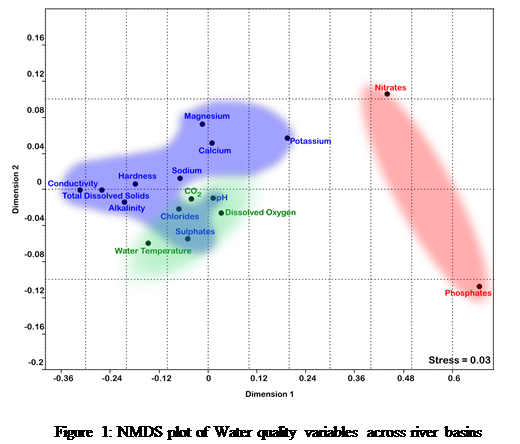
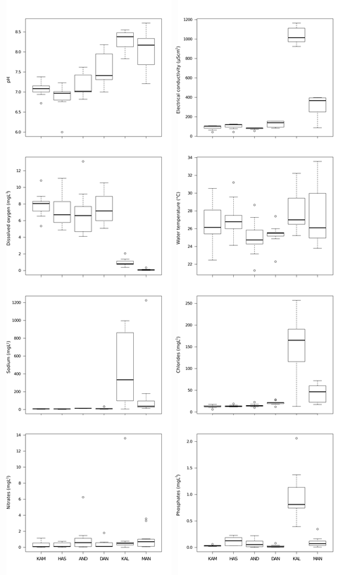
Figure 16: Water chemistry at sampled sites during the study period at BRB
One hundred and three species of diatoms were recorded from all the six sites during the study period, with a flora typical of oligotrophic to eutrophic condition. Among the taxa recored, the most abundant diatom species were Achnanthidium minutissimum (Kϋtz) Czarn., Gomphonema gandhii Karthick & Kociolek, G. difformum Karthick & Kociolek, Nitzschia palea (Kϋtz) W. Sm., Nitzschia frustulum (Kϋtz) Grun., Cymbella sp. and Navicula sp. Achnanthidium minutissimum, Gomphonema gandhii and G. difformum, were present throughout most of the study in LPFS and MPPS, while Nitzschia palea and Nitzschia frustulum were dominant in HPAS. In contrast, Cymbella sp. was the only diatom present at the MAN site during the month of April. The samples from headwater oligotrophic streams (often with low pH and conductivity) were characterized by the occurrence of Gomphonema gandhii, Achnanthidium minutissimum and Gomphonema difformum. Assemblages from eutrophic streams (HPAS) were characterized by dominance of Nitzschia palea, N. frustulum and occasionally with Cyclotella meneghiniana.
The species richness was highest at three sites; KAM, DAN and MAN, even though each one inherited different water chemistry regimes. All six sites were characterized with very low species richness during the monsoon season (Table 3). In all sites across the study, the diversity (H') ranged between the highest 2.34 in DAN during the month of February to lowest of 0 in KAM and KAL during the monsoon months. Kruskal–Wallis results showed that the species diversity across three water chemistry regimes were significantly different (Kruskal–Wallis, H = 6.97; p = 0.03).
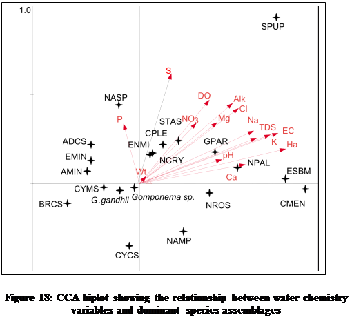
Species abundances across season suggested trends within community composition in ordination space (Figure 18). In sites KAM and KAL communities of post monsoon season aggregated in ordination space, however this trend were not seen in HAS, DAN, MAN and AND sites. In LPFS (KAM and HAS) and MPPS (AND and DAN) diatom assemblages were identical for pre-monsoon, monsoon and post-monsoon seasons respectively, whereas the assemblages in HPAS (KAL and MAN) were not identical across seasons. Though there are trends on community composition, it looks like there is a strong relation with the seasonally dynamic environmental variables. The difference in the species richness among sites were not significant (Kruskal–Wallis H = 6.07; p = 0.29). Species richness from highest to lowest within water quality regimes, followed the order LPFS > MPPS > HPAS. Overall, species richness was lowest during the monsoon months in all the sites. Changes in species composition or percentage turnover (T) did not follow any trend irrespective of site water chemistry. The highest mean turnover (94.44%±11.11) was observed in MAN, indicating the lowest persistence (table 3), followed by DAN (79.08±14.47), HAS (70.46±27.64) and AND (64.77±23.71). The mean species turnover was less than 50% in KAL (47.96±38.1) and KAM (44.03±20.85). Interestingly, KAL showed a wide range of turnover with a minimum of 9% during the post monsoon and a maximum turnover of 100% during the monsoon months. In LPFS sites 25% of the species were persistent across seasons and in MPPS sites 30% of the species were persistent. However in the HPAS sites a minimum persistence of 7.14% was observed for KAL and 80% persistence in MAN. The differences in turnover were significant across sites (Kruskal–Wallis H = 17.52; p = 0.0036).
Table 3: Species richness and diversity across space and time at BRB sites
MONTHS |
LPFS |
HPAS |
MPPS |
KAM |
HAS |
KAL |
MAN |
AND |
DAN |
JAN |
14 (1.10) |
10 (1.04) |
7 (1.58) |
-L- |
4 (0.81) |
14 (2.27) |
FEB |
10 (1.58) |
6(1.10) |
7 (1.65) |
9 (1.63) |
4 (1.04) |
19 (2.34) |
MAR |
4 (1.25) |
6 (0.85) |
8 (1.73) |
14 (1.90) |
6 (0.95) |
-D- |
APR |
7 (1.47) |
7 (0.67) |
9 (1.65) |
1 (0) |
8 (0.93) |
-D- |
MAY |
11 (1.40) |
4 (0.47) |
3 (0.92) |
8 (1.34) |
11 (1.76) |
-D- |
JUN |
9 (1.16) |
3 (0.15) |
4 (1.02) |
-M- |
3 (0.98) |
5 (1.14) |
JUL |
4 (0.77) |
-M- |
1 (0) |
-M- |
6 (1.19) |
7 (1.46) |
AUG |
-M- |
-M- |
-M- |
-M- |
5 (0.79) |
5 (1.35) |
SEP |
1 (0) |
-M- |
1 (0) |
-M- |
2 (0.69) |
9 (1.67) |
OCT |
4 (0.78) |
5 (0.77) |
5 (1.34) |
5 (1.15) |
9 (1.29) |
9 (1.35) |
NOV |
4 (0.82) |
4 (0.94) |
6 (1.54) |
-L- |
-L- |
4 (0.84) |
DEC |
4 (0.87) |
-L- |
8 (1.76) |
16 (2.02) |
2 (0.69) |
10 (1.39) |
Percentage occupancy showed a significant relationship with local maximum species abundance (r = 0.49; P = <0.0001) and local mean species abundance (r = 0.37; P = <0.0001). This positive correlation was slightly stronger for the local maximum abundance; however it was highly significant for both the local abundance measures. Species that occurred locally with more frequency also tended to be abundant across the sites. The species–occupancy frequency distribution (Figure 18) followed a “satellite-mode” (Hanski, 1982) of species distribution, where a high proportion of species occurred at a small number of sites. Sixty-three species occurred in only one site, twenty two species in two sites, eleven species occurred in three sites; five species occurred in four sites, three species occurred in five sites and none of the species occurred in all the six sites.
Diatom Based Biomonitoring
A total of 140 diatom taxa were identified across sites, 61 of them reaching a relative abundance of over 5% in at least one site. Annexure 1 provides the checklist of diatoms. The species compositions were dominated by Gomphonema gandhii Karthick and Kociolek, Achnanthidium minutissimum Kützing, Achnanthidium sp., Gomphonema sp., Gomphonema parvulum Kützing, Nitzschia palea (Kützing) W.Smith, Nitzschia frustulum (Kützing) Grunow var. frustulum, Navicula sp., Navicula cryptocephala Kützing, Cyclostephanos sp., Cymbella sp., Eolimna subminuscula (Manguin) Moser Lange-Bertalot and Metzeltin, Sellaphora pupula (Kützing) Mereschkowksy, Eunotia minor (Kützing) Grunow in Van Heurck, Nitzschia amphibian Grunow f. amphibia, Cyclotella meneghiniana Kützing, Gomphonema difformum Karthick and Kociolek, Navicula rostellataKützing, Cocconeis placentula Ehrenberg var. euglypta (Ehr.) Grunow, Brachysira sp., Stauroneis sp., Encyonema minutum (Hilse in Rabh.) D.G. Mann, Cyclotella sp. and Nitzschia sp. The species composition contains cosmopolitan to possible Western Ghats endemic species and in general species from oligotrophy to highly eutrophic condition were also observed. The current study also documents some of the species for the first time in Western Ghats and many new species descriptions are underway. Waters were circumneutral throughout the whole study area (Table 4), with certain tendency towards alkalinity in the streams drained from agriculture and urban catchment. The highest ionic and nutrient values correspond to the agriculture catchment dominated streams, particularly in the leeward side of the mountains. Oxygenation was generally close to saturation; the lowest values are due to wastewater water inflows in few localities. The most oligotrophic sites were located in mountain watercourses, while downstream sites were generally more polluted, becoming eutrophic in condition. The detailed water chemistry variables are presented in Table 5.
The results of correlation performed between diatom indices and water chemistry variables are presented in the table 6. It is observed that significant correlations exist to varying degrees between most of the diatom indices and water chemistry variables. Diatom indices IPS, EPI and SID showed correlation with more number of water chemistry variables when compared to the other indices. TDI and IPS are negatively correlated with pH, EC, TDS, alkalinity, calcium, magnesium, sodium and potassium. Percent pollution tolerant diatoms were positively correlated with most of the ionic variables. None of the indices were correlated with water temperature. The first four axis of CCA explains 70.1% variance of species-environment relation and the ordination plot reveals two distinct clusters of species.
The species composition contains cosmopolitan to possible Western Ghats endemic species and in general species from oligotrophy to highly eutrophic condition were also observed. Among the species observed in this study, two species were possibly endemic to Western Ghats (G. gandhii, G. difformum and few other species yet to identify). In few sites these species were very dominant reaching more than 80% of the total assemblages. The remaining dominant taxa were cosmopolitan and well documented in international literatures (Krammer and Lange Bertalot, 1986-1991). It is important to note that the indices that were developed and tested in European rivers, lacks Western Ghats endemic taxa. Most sites were oligo-mesotrophic and only a few of the streams were eutrophic. The differences in the water quality of these rivers were reflected in the values for the diatom indices, by the relative abundances of indicators of trophic/saprobic stage and by different types of diatom community.
Table 4: Summary of the Canonical correspondence analysis for the stream sites from Central Western Ghats.
Variables |
Axis order |
1 |
2 |
3 |
4 |
Eigen value |
0.275 |
0.193 |
0.162 |
0.119 |
Species-environment correlations |
0.815 |
0.755 |
0.890 |
0.754 |
Cumulative percentage variance of species data |
10.0 |
17.0 |
22.9 |
27.2 |
Cumulative percentage variance of species-environment relation |
25.8 |
43.8 |
59 |
70.1 |
Table 5: water chemistry variables in 45 sites of CWG streams.
Variables |
Mean |
Std. dev |
Median |
Min |
Max |
pH |
7.22 |
0.49 |
7.14 |
6.03 |
8.16 |
WT (°C) |
25.31 |
2.70 |
25.07 |
19.00 |
33.00 |
EC (µScm-1) |
160.55 |
207.10 |
107.67 |
41.55 |
1164.67 |
TDS (mg L-1) |
122.24 |
204.98 |
60.30 |
20.88 |
1299.67 |
Alkalinity (mg L-1) |
54.55 |
50.32 |
30.00 |
6.81 |
180.00 |
Chlorides (mg L-1) |
32.39 |
40.40 |
22.72 |
5.90 |
220.24 |
Hardness (mg L-1) |
51.26 |
71.05 |
28.00 |
10.00 |
348.00 |
Calcium (mg L-1) |
13.88 |
16.14 |
8.02 |
1.60 |
78.56 |
Magnesium (mg L-1) |
16.35 |
16.73 |
9.36 |
1.17 |
65.95 |
DO (mg L-1) |
6.96 |
1.68 |
7.23 |
2.93 |
10.87 |
Phosphates (mg L-1) |
0.36 |
0.56 |
0.04 |
0.00 |
2.30 |
Nitrates (mg L-1) |
0.74 |
1.10 |
0.13 |
0.03 |
4.30 |
Sulphates (mg L-1) |
25.73 |
20.84 |
16.87 |
0.00 |
74.10 |
Sodium (mg L-1) |
25.77 |
72.18 |
9.09 |
4.11 |
370.00 |
Potassium (mg L-1) |
6.33 |
15.72 |
1.30 |
0.19 |
75.00 |
Table 6: Pearson correlation coefficients between measured water chemistry variables and diatom index scores in 45 sites of CWG streams
INDICES |
pH |
WT |
EC |
TDS |
Alk |
Cl |
Ha |
Ca |
Mg |
Na |
K |
SLA |
-0.33* |
- |
-0.59** |
-0.52** |
-0.49** |
- |
-0.62** |
-0.43** |
- |
-0.51** |
-0.58** |
DESCY |
-0.32* |
- |
-0.54** |
-0.46** |
-0.41** |
- |
-0.65** |
-0.47** |
- |
-0.49** |
-0.52** |
IDSE/5 |
-0.32* |
- |
-0.60** |
-0.50** |
-0.46** |
- |
-0.63** |
-0.45** |
- |
-0.55** |
-0.60** |
SHE |
- |
- |
-0.52** |
-0.38** |
-0.38* |
- |
-0.56** |
-0.41** |
- |
-0.43** |
-0.56** |
WAT |
- |
- |
- |
- |
- |
- |
-0.36* |
- |
- |
-0.34* |
-0.44** |
TDI |
-0.32* |
- |
-0.64** |
-0.54** |
-0.46** |
- |
-0.69** |
-0.53** |
-0.30* |
-0.52** |
-0.58** |
%PT |
0.36* |
- |
0.68** |
0.62** |
0.35* |
0.43** |
0.66** |
0.50** |
0.41** |
0.65** |
0.58** |
GENERE |
- |
- |
-0.49** |
-0.39** |
-0.30* |
- |
-0.54** |
-0.41** |
- |
-0.41** |
-0.41** |
CEE |
- |
- |
- |
- |
- |
- |
-0.36* |
- |
- |
- |
-0.40** |
IPS |
-0.36* |
- |
-0.68** |
-0.59** |
-0.42** |
- |
-0.66** |
-0.46** |
-0.31* |
-0.56** |
-0.58** |
IBD |
- |
|
-0.56** |
-0.43** |
-0.34* |
- |
-0.61** |
-0.46** |
- |
-0.46** |
-0.51** |
IDAP |
- |
- |
-0.51** |
-0.38* |
-0.38* |
- |
-0.56** |
-0.40** |
- |
-0.44** |
-0.53** |
EPI-D |
-0.33* |
- |
-0.58** |
-0.51** |
-0.41** |
-0.31* |
-0.59** |
-0.44** |
- |
-0.53** |
-0.55** |
DI_CH |
- |
- |
-0.54** |
-0.43** |
-0.45** |
- |
-0.58** |
-0.39** |
- |
-0.41** |
-0.53** |
IDP |
- |
- |
-0.48** |
-0.35* |
-0.39** |
- |
-0.58** |
-0.42** |
- |
-0.43** |
-0.49** |
SID |
-0.36* |
- |
-0.50** |
-0.45** |
-0.40** |
-0.38** |
-0.47** |
-0.37* |
- |
-0.43** |
-0.46** |
TID |
- |
- |
-0.53** |
-0.43** |
-0.47** |
- |
-0.59** |
-0.41** |
- |
-0.40** |
-0.48** |
Evenness |
- |
- |
0.39** |
0.40** |
|
- |
0.41** |
- |
- |
- |
- |
Note: WT-Water Temperature, EC-Electric Conductivity, TDS-Total Dissolved Solids, ALK-Alkalinity, Cl-Chlorides, Ha-Total Hardness, Ca-Calcium hardness, Mg-Magnesium hardness, Na-Sodium, K-Potassium. Diatom Indices: SLA-Sládeček’s index, DESCY-Descy’s pollution metric, SHE-Steinberg and Schiefele trophic metric, WAT-Watanabe index, TDI-Tropical diatom Index, GENRE-Generic Diatom Index, CEE-Comission for economical community Index, IPS-Specific Pollution Sensitivity Metric, IBD-Biological diatom index, IDAP-IndiceDiatomique Artois Picardie, EPI-D-Eutrophication/pollution Index, IDP-Pampean Diatom Index,%PT-Percentage Tolerant).
In general, the diatom indices show significant correlations to water quality. The correlations obtained in the present study are comparable to those demonstrated by Taylor et al., (2007c) in South Africa and by Kwandrans et al., (1998), Prygiel and Coste (1993) and Prygiel et al., (1999) in Europe. Significant correlations emphasize that diatom indices can be used to reflect changes in general water quality (Table 6). No correlation of temperature with any of the indices observed that may be due to differing temperature regime in tropical when compared to temperate streams. Similar observation has been recorded by Taylor et al., (2007) from South African rivers. Canonical correspondence analysis (Figure 18) demonstrates that certain widely distributed taxa have similar ecological characteristics in widely separated geographic areas. Species commonly associated with poor water quality in Europe e.g.,Eolimna subminuscula Lange-Bertalot, Nitzschia palea (Kützing) W. Smith, Sellaphora pupula (Kützing) Mereschkowksy, Gomphonema parvulum (Kützing) ordinate on the right hand side of the CCA together with elevated levels of ionic and nutrients. Taxa typical of cleaner, less impacted waters ordinate out on the left hand side of the diagram e.g., Gomphonema difformum Karthick and Kociolek. However Gomphonema gandhii Karthick and Kociolek seems to have a wider ecological tolerance when compared to its morphologically related species. Achananthidium minutissimum group from Western Ghats streams contains morphologically three distinct taxa with wide ecological preferences. Despite the reevaluation of this genus multiple times (Lange-Bertalot and Krammer, 1989, Krammer and Lange-Bertalot, 1991, Potapova and Hamilton, 2007) there are still major gaps in taxonomy and ecology apart from non-inclusion of specimens from tropical rivers. The similar problem holds good for some of the other genus like Gomphonema. This analysis helps to demonstrate that the widely distributed species encountered in the streams of Western Ghats which are not identical only with morphology also have similar environmental tolerances G. gandhii and G. difformum are one among the dominant taxa in this data set but not included in any of the index calculations and their omission could result in an under or overestimation of the index scores. Taylor et al., (2007d) cautioned about the associated problems with usage of European indices in South African rivers. These suggest that European diatom indices can be used in India provided indices address the issues concerned with ecology of endemic species. Hence, the list of taxa included in the indices needs to be adapted according to the study region with giving more importance to the local endemic flora which encourages taxonomic and ecological studies in tropics. The structure of benthic diatom communities and the use of diatom indices yield good result in water quality monitoring in India. It is also evident from the current study that many widely distributed diatom species have similar environmental tolerances to those recorded for these species in Europe and elsewhere. However, the occurrence of possible endemic species will necessitate the work towards diatom index unique to India. In the mean time considerable amount of importance should be paid for taxonomic and ecological understanding of endemic flora for development of improved biomonitoring program.
LULC Analysis: LULC showed considerable variability among catchments, with forest/vegetation land cover as a dominant class (mean = 64.36%, range = 0.13–95.45%), followed by agriculture/cultivation area (mean = 24.27% range = 2.55-63.63%), among the 24 catchments. LULC analysis shows that natural vegetation is poor towards the leeward side of the mountains (eastern region), due to intense anthropogenic activities. This region has more of agriculture, open scrub/barren land, and built-up area. In the entire study region the class forest/vegetation covers predominantly moist deciduous type, with small isolated patches of semi-evergreen vegetation in the eastern region and the western region (windward side) with rugged hilly terrain and heavier rainfall (~5000 mm) having characteristic evergreen to semi-evergreen forests. The detailed LULC for each catchment is given in the Table 7 and the land cover images are given in Figure 19. The dendrogram of sites based on LULC obtained by Ward's method is shown in Figure 20. Three well differentiated clusters can be seen, with forest cover decreasing and agriculture/cultivable land cover increasing from top to bottom. The third cluster from top includes sites SAN, KAL, MAN, SAP and GUN, which are characterized with high amount of agricultural activities (>50%). The group in center is characterized by more forest cover (>50%) with moderate amount of agricultural land. Another top most group is dominated by forest land cover of more than 80%.
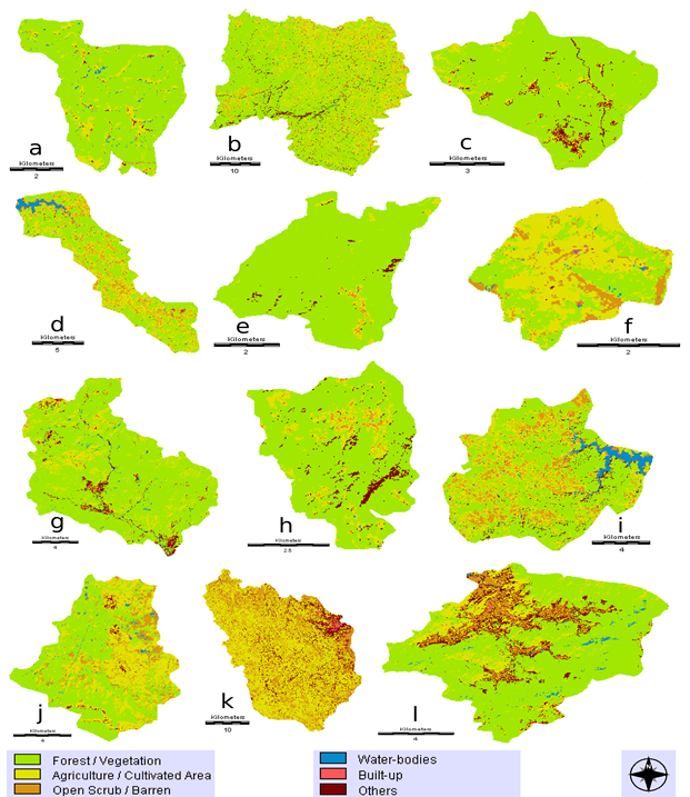
Figure 19: Classified land use images of study catchments in Central Western Ghats. a - Daanandhi, b - Deevalli, c - Badapoli, d - Mavinahole, e - Makkegadde, f - Gunjavathi, g – Sakathihalla, h – Angadibail, i – Hurlihole, j – Chitgeri, k - Kalghatghi, l – Naithihole
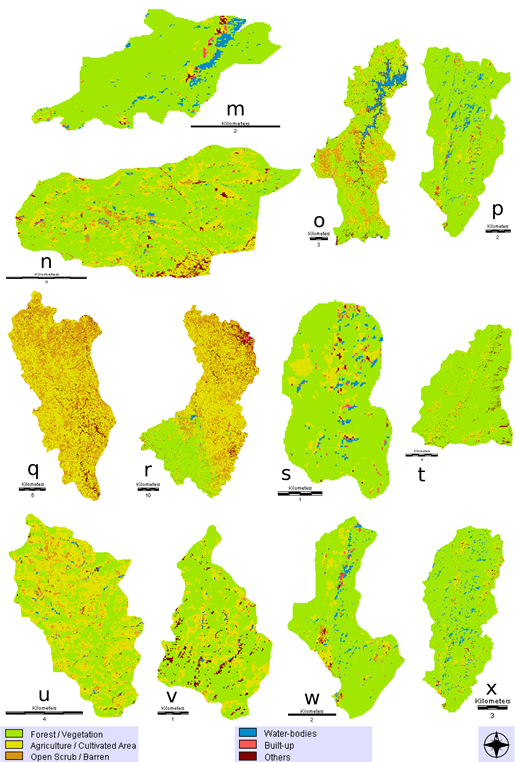
Figure 19 (cont.): Classified land use images of study catchments in Central Western Ghats. m - Beegar, n - Andhalli, o – Yennehole, p - Kammani, q - Sangadevarakoppa, r - Machikere, s - Melinakeri, t - Yanahole, u - Sapurthi, v - Bailalli, w - Kelaginakere, x – Hasehalla
Water Chemistry: Water chemistry was characterized by high spatial variability in nutrients and ionic strength among the 24 sites. Nutrients like nitrates showed a many fold variability from 0.07 to 4.24 mgL-1. Sites in the mountain range and wind ward side were characterized by low nutrient and ionic variables; where as the sites on the lee ward sides of the mountains were characterized with high nutrients, ions and low dissolved oxygen levels. The dendrogram of sites based on the water chemistry is shown in Figure 20. Two well differentiated clusters can be seen, with sites containing moderate to low levels of nutrient and ions in the top cluster and two severely polluted sites at bottom. The top cluster further divide in to four sub cluster based on the ionic and nutrient values. Clustering of most of the sites in cluster based on water chemistry variables are similar to the cluster of sites based on the land cover variables. A PCA bi-plot of water quality variables and LULC for all sample sites is given in Figure 21. The two-dimensional bi-plot describes 65% of the variation in data, where 52% displayed on the first axis and 13% is displayed on the second axis. Among water chemistry variables, ionic variables were positively correlated with first axis and among the LULC variables percentage agriculture and scrub land cover were positively related to the first axis. Sites with more than 50% of agriculture land cover were separated from other sites on the PC2 axis indicating trends in water quality may be related to land use. Agriculture dominated sites were placed due to the higher conductivity, ionic and nitrates levels relative to the forest dominated sites, which are characterized by low ionic and nutrient in nature.
Diatom Assemblages:
Among the 113 taxa the most common and dominant diatom taxa are Eolimna subminuscula, Achnanthidium sp., Navicula sp., Nitzschia palea, Gomphonema parvulum, Gomphonema sp., Gomphonema gandhii, Achnanthidium minutissima and Cyclostephanos sp. The list of species with their abundance is presented in the Appendix 1. Species richness varied from 4 to 29 with an average of 15. Shannon-Wiener diversity varied from 0.71 to 2.94 with an average of 1.76. According to the pH classification, diatom assemblages were characterized by a high proportion of neutrophilous diatom species (64.62%) followed by alcaliphilous species (26.64%). Salinity classification based on the diatom species assemblages infer the fresh to brackish water species were the dominant form with 86.16% followed by brackish to freshwater (7.84%) and exclusively freshwater (5.3%) flora.
Nitrogen autotrophic taxa, which tolerate elevated concentrations of organically bound nitrogen, were dominant with 53.31%. Species which require 100% oxygen saturation were prevailing community with 42.98% followed by low level (30% oxygen saturation) oxygen requirement species by 29.08%. The composition of diatom community with respect to saprobity in the order or oligosaprobous, β-mesosaprobous, α-mesosaprobous, α-meso-/polysaprobous and polysaprobous were 7.8%, 46.09%, 10.58%, 26.56% and 8.97% respectively. The species occurs in the eutraphentic and oligo to eutraphentic were equally dominant with respect to the trophic state explained by diatoms. <
Relationship of LULC with water chemistry and diatom assemblages
Correlation between percentage agricultural land cover with water chemistry variables and diatom autecological indices revealed the role of landscape level drivers in natural forest cover due to creation of new settlement for relocation of people and associated increase in cultivation of crops (Hegde et al., 1994). Earlier studies confirm that agricultural expansion as one of the major driver for deforestation (Menon and Bawa, 1998) in Western Ghats determining the environmental condition of streams and diatom assemblages (Figure 22). The gradient of percentage agriculture land cover were positively correlated with water chemistry variables like electrical conductivity (r = 0.67), total dissolved solids (r = 0.62), nitrates (r = 0.60) and pH (r = 0.52). Gradient of percentage agriculture land cover were positively correlated with percentage pollution tolerant diatoms (r = 0.65, Figure 23). Relation between the diatom autecological indices with land cover and water chemistry variables are given in Tables 7 and 8 respectively. Most of the diatom autecological parameters were positively correlated with forest/vegetative cover and negatively correlated with agriculture/cultivable and scrub land cover. All the diatom indices were normalized to a range of 0-20, where <9 indicates bad water quality, 9 to 12 indicates poor water quality, 12 to 15 indicates moderate water quality, 15 to 17 indicates good quality and >17 indicates high quality. The present study shows that within a similar ecoregion, the diversity and community composition of diatoms changes with LULC pattern. Among all the 24 catchments, most of the catchments were dominated by forest/vegetation land cover. However, forest cover in the leeward side catchment was very low owing to anthropogenic activities. Hydro power projects commenced in the study area since 1960s seem to have lost.
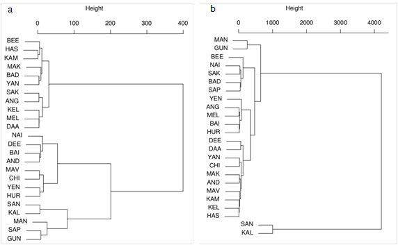
Figure 20: Dendrogram of the cluster analysis based on (a) LULC and (b) water quality, according to the 24 sampling sites of the Central Western Ghats
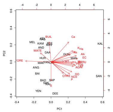
Figure 21: PCA bi-plots of water chemistry and LULC variables in study sites in Central Western Ghats streams
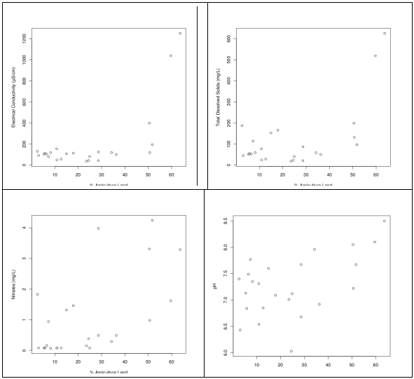
Figure 22: Changes in water quality variables along a gradient of percentage agricultural land cover in Central Western Ghats.
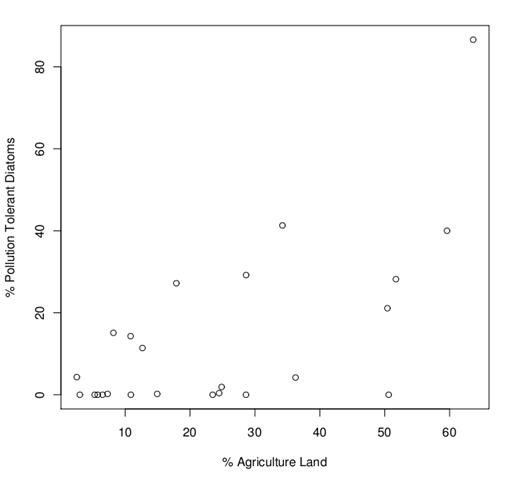
Figure 23: Relations between percentage pollution tolerant diatoms with gradient of percentage agricultural land cover in Central Western Ghats
The streams drained from catchment with agriculture and scrub land cover were characterized with ionic and nutrient rich, which notify that the water chemistry variables were decided by the land cover types. Many studies have reported that urban and agricultural land use play a primary role in degrading water quality in adjacent aquatic systems by altering the soil surface conditions, increasing the impervious area and generating pollution (Tong and Chen, 2002; White and Greer, 2006).
Table 7: Percentage LULC classes for each catchment in the study area
|
Forest/ Vegetation |
Agriculture/ Cultivation |
Open Scrub/ Barren Land |
Water Bodies |
Built Up |
Others |
CHI |
52.5 |
34.24 |
10.9 |
1.18 |
0.14 |
1.04 |
MEL |
83.58 |
10.88 |
0.57 |
2.84 |
1.52 |
0.61 |
KEL |
85.83 |
8.19 |
1.4 |
3.03 |
0.92 |
0.62 |
BEE |
90.41 |
2.55 |
0.16 |
5.11 |
1.16 |
0.61 |
ANG |
81.54 |
12.67 |
1.38 |
0.08 |
0.18 |
4.14 |
MAK |
95.45 |
3.02 |
0.38 |
0.01 |
0.13 |
1.01 |
HUR |
52.84 |
28.62 |
11.89 |
3.91 |
0.1 |
2.64 |
MAV |
48.85 |
36.26 |
10.79 |
2.94 |
0.43 |
0.73 |
YEN |
56.15 |
24.49 |
10.47 |
5.61 |
0.16 |
3.12 |
BAI |
70.85 |
23.49 |
0.99 |
0.58 |
0.2 |
3.89 |
DEE |
64.34 |
28.64 |
3.62 |
0.51 |
0.2 |
2.69 |
YAN |
90.83 |
6.52 |
0.56 |
0.02 |
0.08 |
1.98 |
SAP |
42.8 |
50.61 |
4.5 |
0.97 |
0.31 |
0.81 |
BAD |
88.36 |
7.29 |
0.24 |
0.11 |
0.06 |
3.94 |
NAI |
67.43 |
17.89 |
3.65 |
1.03 |
0.44 |
9.58 |
SAK |
80.08 |
14.94 |
0.26 |
0.92 |
0.24 |
3.58 |
AND |
68.1 |
24.87 |
3.36 |
0.93 |
0.98 |
1.77 |
DAA |
86.29 |
10.84 |
0.58 |
1.26 |
0.41 |
0.63 |
HAS |
88.6 |
5.77 |
0.42 |
3.96 |
0.88 |
0.37 |
KAM |
88.8 |
5.31 |
0.6 |
4.01 |
0.89 |
0.39 |
MAN |
23.46 |
50.42 |
20.69 |
0.67 |
0.52 |
4.25 |
KAL |
0.53 |
59.6 |
30.22 |
0.02 |
0.84 |
8.79 |
SAN |
0.13 |
63.63 |
31.48 |
0.02 |
0.16 |
4.59 |
GUN |
36.82 |
51.72 |
10.52 |
0.52 |
0.35 |
0.07 |
The results suggest better water quality tendencies in watersheds having less urbanization with more natural vegetation region. Percent agriculture in the catchment ranged from 2 to 63% with an average of 24.27% so the sites we selected covered a good range of the land-use gradient. An aggregated measure of LULC such as percentage agriculture in catchments may only represent the potential of LULC effects on streams. Percentage agriculture lands in catchments were positively correlated with the ionic and nutrient variables. Studies have shown that the percentage of agriculture at watershed scale is a primary predictor for nitrogen and phosphorus (Ahearn et al., 2005).
Table 8: Water chemistry variables of the sampling sites in Central Western Ghats
Water Chemistry variables (Units) |
Mean±S.D |
Range |
pH |
7.28±0.58 |
6.03-8.50 |
Water Temperature (°C) |
26.09±2.52 |
22.10-35.43 |
Electrical Conductivity (µScm-1) |
199.00±301.44 |
37.17-250.67 |
Total Dissolved Solids (mgL-1) |
120.26±149.68 |
18.67-624.67 |
Alkalinity (mgL-1) |
70.44±111.46 |
12.00-421.07 |
Chlorides (mgL-1) |
35.25±62.36 |
4.99-255.92 |
Hardness (mgL-1) |
69.49±96.94 |
12.00-376.00 |
Calcium (mgL-1) |
14.76±17.33 |
1.60-84.97 |
Magnesium (mgL-1) |
15.72±18.58 |
1.17-71.01 |
Dissolved Oxygen (mgL-1) |
7.58±1.77 |
4.81-11.52 |
Phosphates (mgL-1) |
0.18±0.36 |
0.01-1.30 |
Sulphates (mgL-1) |
19.94±18.07 |
2.91-67.91 |
Sodium (mgL-1) |
52.92±201.09 |
1.05-996.03 |
Potassium (mgL-1) |
11.01±35.01 |
0.41-168.33 |
Nitrates (mgL-1) |
1.06±1.33 |
0.07-4.24 |
Diatom community structure in streams of the CWG was strongly related to land use practices as in many other regions (Stevenson et al., 2009; Walsh and Wepener, 2009). The nutritional changes in the streams triggered by the LULC analysis stands as a determining factor in structuring the diatom species composition. Effects of nutrient are commonly identified as one of the most important determinants of diatom species composition in lentic and lotic ecosystems (Pan and Stevenson, 1996). However the diatom species composition at CWG stream were controlled more by the ionic variables than the nutrient concentration, which is evident by the dominance of fresh to brackish water diatom species in agriculture catchments. More of pollution tolerant species were seen in the streams in agriculture dominated catchments. Blinn (1993, 1995) found that higher salinities (≥35 mScm-1) tend to override other water quality parameters in structuring diatom communities in salt lakes. Agriculture dominated sites like SAN and KAL represented water quality with high nutrient concentration along with elevated levels of total dissolved solids, and pH (Figures 22 and 23) which is also supported by positive correlation of percentage agriculture land cover with percentage pollution tolerant diatoms (Figure 23). Correlation analyses between measured land cover of the watersheds and water quality parameters reveal a number of interesting aspects of the pattern effects of land uses on water quality. The application of indices on the diatom communities revealed significant correlation of only percent pollution tolerant diatoms with land use variables. The significant positive correlation of all the water chemistry variables with agriculture land use represents more human induced activities, whereas water temperature did not correlate significantly with any of the variables. This may be due to varying depth and different water regimes (Taylor, 2004). As would be expected streams in catchments with intensive agriculture were characterized by increased concentrations of nutrients and ions, which is evident from the principal component analysis. Clear differences in community composition were seen in NMDS analysis, where diatom community from streams with agriculture land cover was clustered out separately, except one site. According to NMDS analysis, diatom communities were significantly different in streams with different catchment nature. Diatom community in the forested streams were dominated by endemic diatom flora (Gomphonema gandhii Karthick and Kociolek, G. difformum Karthick and Kociolek, G. diminutum Karthick and Kociolek and many unidentified species from genus Navicula), whereas the streams from agricultural dominated landscapes were dominated by cosmopolitan species (Gomphonema parvulum Kützing, Nitzschia palea (Kützing) W.Smith, Achnanthidium minutissima Kützing v. minutissima Kützing).
|

