Parameters	Units	Methods	Section no. APHA,  1998.
pH	-	Electrode Method	4500-H+ B
Water Temperature	ºC		2550 B
Salinity	ppm		2520 B
Total Dissolved Solids	ppm		2540 B
Electrical Conductivity	µS		2510B
Dissolved Oxygen	mg/L	Iodometric method	4500-O B
Alkalinity	mg/L	HCl  Titrimetric Method	2320 B
Chlorides	mg/L	Argentometric Method	4500-Cl- B
Total Hardness	mg/L	EDTA Titrimetric Method	2340 C
Calcium Hardness	mg/L	EDTA Titrimetric Method	3500-Ca B
Magnesium Hardness	mg/L	Calculation Method	3500-Mg B
Sodium	mg/L	Flame Emission Photometric Method	3500-Na B
Potassium	mg/L	Flame Emission Photometric Method	3500-K B
Fluorides	mg/L	SPADNS method	4500-F- D
Nitrates	mg/L	Nitrate Electrode method and Phenol Disulphonic Acid Method	4500-NO3- D
Sulphates	mg/L	Turbidimetric method	4500-SO42- E
Phosphates	mg/L	Stannous Chloride Method	4500-P D

Diatom Collection, Preparation and Enumeration: Figure 7 illustrates the habitat of diatoms – diatom colonies on stones, sand, etc. At each site, three to five stones were randomly selected across the stream and diatoms were scraped off the exposed surface of the stones using a tooth brush. Fresh samples were carefully checked to assure that majority of the diatom frustules were alive prior to acid combustion. A hot HCl and KMnO4 method was used to clean frustules of organic materials. The cleaned diatom samples were dried on 18x18 mm cover slips and mounted with Pleurax. A total of 400 frustules per sample were enumerated and identified using compound light microscope (Lawrence & Mayo LM-52-series, with 1000× magnification) following methods described by Taylor et al. (2005) and Karthick et al. (2010). Diatoms were identified primarily to the species level according to Gandhi, (1957a,b,c; 1958a,b; 1959a,b,c; 1960a,b,c); Krammer and Lange-Bertalot (1986–1991) and Taylor et al. (2007).

 

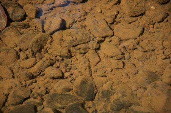
Figure 7: Diatoms on stone in streams

 

Land Use Land Cover (LULC) Analysis

The remote sensing data are processed to quantify the land use of respective basins broadly into 6 classes – forest and vegetation; agriculture and cultivated area; open scrub and barren; water bodies; built-up; and others (includes categories like rocky outcrop, etc.). The multi-spectral data of Indian Remote Sensing (IRS) LISS-III with a spatial resolution of 23.5m were analyzed using IDRISI Andes (Eastman, 2006; http://www.clarklabs.org) and GRASS (http://ces.iisc.ernet.in/grass).  Land use analysis involved i) generation of False Colour Composite (FCC) of remote sensing data (bands – green, red and NIR). This helped in locating heterogeneous patches in the landscape ii) selection of training polygons (these correspond to heterogeneous patches in FCC) covering 15% of the study area and uniformly distributed over the entire study area, iii) loading these training polygons co-ordinates into pre-calibrated GPS, vi) collection of the corresponding attribute data (land use types) for these polygons from the field . GPS helped in locating respective training polygons in the field, iv) supplementing this information with Google Earth (http://www.googleearth.com)  v) 60% of the training data has been used for  classification, while the balance is used for validation or accuracy assessment. Based on these signatures, corresponding to various land features, supervised image classification was carried out using Gaussian Maximum Likelihood Classifier (GMLC) to the final six categories.

Data Analysis :

Compiled data were tested for normality before performing statistical analyses. Statistical analyses comprised Kruskal-Wallis test (H), Principal Component Analysis (PCA) and Non-Metric Multi Dimensional Scaling (NMDS).  All tests were performed using the R-software (R Development Core Team, 2006).Box plots are used throughout this report to visually summarize data. These graphs depict the following statistical measures: median, upper and lower quartiles. The box plot is interpreted as follows: The box itself contains the middle 50 percent of the data. The upper edge of the box indicates the 75th percentile of the data set, and the lower edge of the box indicates the 25th percentile. The line in the box indicates the median value of the data. If the median line within the box is not equidistant from the edges of the box, then the data are skewed. “Gridding” is the operation of spatial interpolation of scattered 2D data points onto a regular grid. Gridding allows the production of a map showing a continuous spatial estimate. The spatial coverage of the map is generated automatically as a square covering the data points. Non-metric multidimensional scaling is based on Bray-Curtis distance matrix was performed for classifying the sites across river basins. In NMDS, data points are placed in 2 or 3 dimensional coordinates system preserving ranked differences.

Data were tested for normality before performing statistical analyses. Statistical analyses comprised Kruskal-Wallis test (H), Principal Component Analysis (PCA) and Non-Metric Multi Dimensional Scaling (NMDS).  All tests were performed using the R-software (R Development Core Team, 2006). The non-parametric Kruskal-Wallis test was used to assess whether species richness, species diversity and turnover across water quality regimes were significantly different. Temporal variation in diatom assemblages in each site was analyzed by NMDS using absolute abundance data. NMDS is an ordination method well suited to data that are non-normal or are arbitrary or discontinuous and for ecological data containing numerous zero values (Minchin, 1987; McCune & Grace, 2002). Results were visualized showing the most similar samples closer together in ordination space (Gotelli & Ellison, 2004). A final stress value, typically between 0 and 15, was evaluated as a measure of fitted distances against the ordination distance, providing an estimation of the goodness-of-fit in multivariate space. Changes in species composition or percentage turnover (T) were used to indicate community persistence. T was calculated as T=(G + L)/(S1 + S2) times 100 where G and L are the number of taxa gained and lost between months respectively, and S1 and S2 are the number of taxa present in successive sampling months (Diamond & May, 1977; Brewin et al. 2000; Soininen & Eloranta, 2004). The relationship between local population persistence, local abundance in terms of relative abundances, and regional occupancy were examined using correlation analysis (Soininen & Heino, 2005). For the species distribution model the species were classified as core species as species that occurred in over 90% of sites, and satellite species as species that occurred in fewer than 10% of sites (McGeoch & Gaston, 2002, Soininen & Heino, 2005). Local occupancy of each diatom species was calculated by their percentage of occurrence at each site across the seasons. Seasonal diatom community was related to the water quality parameters using multiple linear regressions. Finally, water quality variables were used in PCA to elucidate the spatial water quality variation.