Multiple data sources from various agencies were used in order to evaluate the hydrological scenario of the Varada River. Table1 describes the various data sources used for assessment of the hydrological regime across the catchments.

Table 1: Data

METHOD:

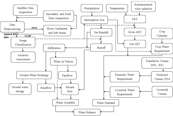
Figure 5: Method involved

The method involved in evaluation of the hydrological status is as depicted in figure 5. The process of evaluation involves 1) extraction of catchment boundary 2) land use analysis, 3) assessment of the hydro meteorological data, 4) analysis of population data, 5) public interactions 6) water requirement for domestic and agriculture/horticulture, 7) assessment of the hydrological status.
Extraction of catchment boundary: Catchment boundaries and the stream networks considering the topography of the terrain based on Cartosat DEM were extracted using the hydrologic modeling tool in GRASS GIS. Since DEM has inherent errors, the catchment boundaries were overlaid on the extracted boundaries from survey of India toposheets in order to check and correct the variations, these corrected catchment boundaries were further overlaid on Google earth in order to visualize the terrain variations more precisely (fig 1).
Land use Assessment: Land use refers to heterogeneous terrain with the interacting ecosystems and is characterized by its dynamics, which are governed by human activities and natural processes. Human induced land use and land cover (LULC) changes have been the major driver of the landscape dynamics at local levels. Land use assessment was carried using the maximum likelihood classification technique. Understanding of landscape dynamics helps in the sustainable management of natural resources. The process of assessing land use is as follows:

• Satellite data acquisition: Satellite data sets for the whole world (earth) at different resolutions are available since 1972 (Landsat1) up to date. For the land use analysis, Landsat 8 (2013) data was obtained from the public domain (USGS: earthexplorer.usgs.gov/).   
• Data pre processing: Since the satellite data could contain errors such as shift (geometric errors) or erroneous pixels (radiometric errors), correction are applied on each band. Radiometric corrections involve contrast enhancement, elimination of noise etc. Geometric corrections involve precisely referencing the satellite data with the help of field data from GPS, Google earth, Toposheet or Bhuvan.
• Preparation of False Colour Composite: False colour composite is the representation of earth features in their non-original colours in order to identify the heterogeneity in various land scapes. FCC are prepared by combination of various spectral bands such as the NIR, GREEN and RED bands.
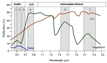
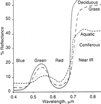
• Preparation of signature data set: Signatures are the training datasets which are used to classify the satellite image into various land use classes based. Signatures are developed for various land use categories based on the site knowledge (Field data, Toposheets, Google earth, Bhuvan, Western Ghats Biodiversity Portal, French institute maps) and based on spectral reflectance characteristic (fig. 6) of different land scape. Training data should be unique and homogeneously spread across the study area covering at least 15% of the total area.

Figure 6: Spectral reflectance curve

• Classification of remote sensing data (Satellite images): Classification process is carried out using the Gaussian maximum likelihood classifier. The classifier computes the mean and variance of digital numbers under each training data set, based on which new pixel is categorized under a land use class. Of the overall signatures, 65% of the total signatures are considered in classification of the image and 35% of the pure signatures are used for assessing the accuracy.

• Accuracy assessment: Accuracy is necessary in order to check if the classified satellite data agrees with that of the reference data. The reference data can be obtained based on the field data, or any other map. Kappa is estimated as a measure of agreement between the reference map and the classified map.

Assessment of the hydro meteorological data: This process involves assessment of the rainfall data obtained from various sources such as TRMM, Rain gauge stations in and around the study site. Based on the long term precipitation data are used in order to understand rainfall variation over decades. Isolines across the months were developed based on the spatial rainfall variation of rainfall w.r.t the raingauge stations across the basin. Along with rainfall, temperature (minimum, maximum and average), extra-terrestrial solar radiation across the catchment were used to hydrological behaviors of the catchments which enables to understand the hydrological status.
Rainfal: Point based daily rainfall data from various rain gauge stations in and around the study area between 1901 and 2010 were considered for analysis of rainfall. The rainfall data used for the study were obtained from

• Department of statistics, Government of Karnataka
• Indian metrological data (IMD), Government of India
• Tropical rainfall Measuring Mission (TRMM), NASA

Since some rain gauge stations had incomplete records with rainfall missing for few months, analysis without these data would yield erroneous results and also stations with missing rainfall cannot be included in the analysis, which otherwise would give better representation of the results, these missing data’s were evaluated through regression analysis and error data’s were revised with respect to neighboring rain gauge stations. Rainfall trend analysis was observed for selected rain gauge stations to assess the variability of rainfall at different locations in the study area.

The points based long term daily rainfall data were used to calculate the monthly and annual rainfall in each rain gauge station based on mean and standard deviation of rainfall at selected rain gauge stations. The average monthly and annual rainfall data were used to derive rainfall throughout the study area through the process of interpolation (isohyets). The interpolated rainfall data was used to derive the gross yield (RG) in the basin. Net yield (RN) was quantified as the difference between gross rainfall and interception (In).

RG = A * P
RN = RG – In

Where
RG  :   Gross rainfall yield volume, A :   Area in Hectares,  P :  Precipitation in mm
RN :  Net rainfall yield volume, In :  Interception volume

Run off: This is the portion of rainfall that flows in the streams after precipitation. Runoff can be typically divided into two categories i) Surface runoff or Direct Runoff ii) Sub surface runoff
Surface Runoff: Portion of water that directly enters into the streams during rainfall. Surface runoff in the region is estimated based on the empirical equation (eq1)

Q = Σ(Ci*PR*Ai)

Where Q : Runoff in cubic meters per month
C : Runoff Coefficient which is dependent upon various land uses (table 2)
PR : Net rainfall in mm ( Gross rainfall – Interception)
i : Land use type  
Table 2: Runoff Coefficients

Interception: During monsoons, portion of rainfall falls doesnot reach the surface of the earth, it remains on the canopy of trees, roof tops, etc. this portion of water is lost in the process of evaporation. Studies show that, losses due to interception is over 15% to 30%, based on the land use. Table 3 shows the interception loss across various rainy months and land uses
Table 3: Interception loss

Infiltration: Due to precipitation, apart from surface runoff and interception, the remain portion of water enters the subsurface of the earth saturating the sub soils, and percolating into the ground water table and hence recharging ground water. The infiltered water enters the streams during post monsoon, as pipe flow and baseflow.

Inf = RN - Q

Ground water recharge:
This is the portion of water that is percolated below the soil stratum (vadose) after soil gets saturated. Recharge is considered the fraction of infiltrated water that recharges the aquifer after satisfying available water capacity and pipe flow. Krishna Rao equation (1970) was used to determine the ground water recharge. 

GWR = RC * (PR – C) * A

Where 
GWR   : Ground water recharge
RC        : Ground water recharge coefficient (table 4)
C         : Rainfall Coefficient
A         : Area of the catchment

The recharge coefficient and the constant vary from location to location based on the annual rainfall.
Table 4: Ground water recharge coefficients

Sub Surface Flow (Pipeflow): Pipeflow is considered to be the fraction of water that remains after infiltrated water satisfies the available water capacities under each soil. Pipe flow is estimated for all the basins as function of infiltration, ground water recharge and pipeflow coefficient, i.e.,

PF = (Inf – GWR) * KP

Where 
PF        : Pipeflow
Inf       : Infiltration volume
KP        : Pipeflow coefficient
Groundwater Discharge: Groundwater discharge or baseflow is estimated by multiplying the average specific yield of aquifer under each land use with the recharged water. Specific yield represents the water yielded from water bearing material. In other words, it is the ratio of the volume of water that the material, after being saturated, will yield by gravity to its own volume. Baseflow appears after monsoon and pipeflow has receded. This water generally sustains flow in the rivers during the dry season.

GWD = GWR * YS

Where
GWD = Ground water discharge
GWR   = Ground water recharge
YS        = Specific yield

Evapotranspiration: Evaporation is a process where in water is transferred to atmosphere as vapour from open waters, whereas Transpiration is the process by which water from plants through leaves and other parts above ground. In the process of transpiration water is taken into the atmosphere from ground (soil) through the roots. On the other hand, evaporation continues throughout the day and night at different rates. The process of evaporation takes place on all different land uses other than vegetation. Evapotranspiration is the total water lost from different land use due to evaporation from soil, water and transpiration by vegetation.

Some of the important factors that affect the rate of evapotranspiration are:

• Temperature
• Wind
• Light intensity
• Sunlight hours
• Humidity
• Plant characteristics
• Land use type
• Soil moisture

If sufficient moisture is available to completely meet the needs of vegetation in the catchment, the resulting evapotranspiration is termed as potential evapotranspiration (PET). The real evapotranspiration occurring in specific situation is called as actual evapotranspiration (AET). These evapotranspiration rates from forests are more difficult to describe and estimate than for other vegetation types.

Potential evapotranspiration (PET) is determined using Hargreaves method (Hargreaves, 1972) an empirical based radiation based equation, which is shown to perform well in humid climates. PET is estimated as mm using the Hargreaves equation is given as

PET = 0.0023 * (RA/λ) *  *

Where           

RA        = Extra-terrestrial radiation (MJ/m2/day) (FAO)
Tmax   = Maximum temperature
Tmin    = Minimum temperature
λ          = latent heat of vapourisation of water (2.501 MJ/kg)

Actual evapotranspiration is estimated as a product of Potential evapotranspiration (PET) and Evapotranspiration coefficient (KC) (table 5), the evapotranspiration coefficient is a function of land use varies with respect to different land use. Table 5 gives the evapotranspiration coefficients for different land use

AET = PET * KC
Table 5: Evapotranspiration coefficient

*As the crop water requirement was estimated for different crops and different seasons based on land use, assumption is individual crop water requirement based on their different growth phases need different quantum of water for their development inclusive of evaporation.*

Analysis of population data and domestic water demand: Population dynamics in any region is necessary in order to understand and predict the domestic water demand. Population census for the year 2001 and 2011at village lever were considered in order to derive the population of the basin level. Based on the rate of change of population , the population for the year 2014 was predicted.

r = (P2011/P2001 – 1)/n

Where
P2001 and P2011 are population for the year 2001 and 2011 respectively
n is the number of decades which is equal to 1
r is the rate of change

P2014 = P2011 * (1 + n*r)

Where
P2014 is the population for the year 2014
n is the number of decades which is equal to 0.3
Domestic water demand is assessed as the function of water requirement per person per day, population and season. Water required per person include water required for bathing, washing, drinking and other basic needs. Water requirements across various seasons are as depicted in table 6
Table 6: Seasonal water requirement

Data collection from public and Livestock water requirement: Public interviews were conducted in order to understand the agricultural cropping pattern and water needed for various crops in the catchment, livestock census was obtained from the district statistics and water requirement for different animals were quantified based on the interviews. Table 7 gives the various livestock water requirements
Table 7: Livestock water requirement

Crop water requirement: Based on the crops grown and cropping pattern in the catchment according to the district at a glance, department of agriculture assisted by the public interviews, the crop water requirement was estimated for various crops based on their growth phases. Land use information was used in order to estimate the cropping area under various crops. Table 8 provides the information of various crop water requirements based on their growth phase as cubic meter per hectare for Sagara Taluk.
Table 8: Crop water requirement

Assessment of the hydrological status: The hydrological status in the catchment is analysed for each month based on the water balance which take into account the water available to that of the demand. The water available in the catchment is function of water available in the water bodies such as lakes, streams and rivers, water in the soil, pipe flow and base flow, whereas the demand in the catchment is estimated as the function of crop water demand, domestic and livestock demand and the evapotranspiration waters. The catchments is said to be stable if the water available caters the water demand completely else the catchment is devoid of water and would lead to drought like conditions in the catchment.