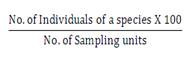
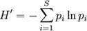
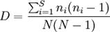
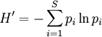
Methods and Materials

Diatom sampling

Diatom samples were collected (from cobbles, aquatic plants and sediment) and prepared using standard methods as per Taylor et al., (2005) from selected wetlands. Diatom communities were then analysed by counting between 400 and 450 valves. During enumeration the dimensions of diatom valve characteristics, like its length, width and straie densities in 10 µm were measured. Identification of diatoms is carried out using taxonomic guides (Gandhi, 1957 1959a, 1959b, 1961, 1962, 1967, 1998; Lange-Bertalot, 2001; Krammer, 2002; Taylor, 2007; Karthick et al., 2008).

Water samples were collected from all sites and physical variables like pH, temperature, Electric conductivity, Salinity and Total dissolved solids were measured using EXTECH combo probe.  

Ecological diversity was calculated for each sample using diversity indices given in Table 1.

Table 1 : Diversity parameters and indices

Index	Equation	Remarks	References	Eq.No
Abundance				1
Shannon Weiner’s (H’)	Pi: proportion of individuals of ith species	The value ranges between 1.5 and 3.5 and rarely surpasses 4.5	Ludwig and Renolds (1998); Legendre and Legendre 1998	2
Simpson’s		The value varies from 0 to 1. A value of 0 indicates the presence of only one species, while 1 means that all species are equally represented.	Ludwig and Reynolds (1998)	3
Dominance	1-Simpson index D = sum Where ni is number of individuals of taxon i.	The occupancy of a species over an area. Ranges from 0 (all taxa are equally present) to 1 (one taxon dominates the community completely)		4
Evenness		The measure of biodiversity which quantifies how equal the community		5
Fisher's alpha	Where S is number of taxa, n is number of individuals and a is the Fisher's alpha.	It is a mathematical model used to measure diversity		6
Berger-Parker	Where Nmax is the number of individuals in the most abundant species and N is the total number of individuals in the sample.	The number of individuals in the dominant taxon relative to n, where n is the total number of species	Berger and Parker 1970;	7

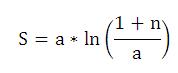
Diatom specific indices like Generic Diatom Index or GDI (Coste and Ayphassorho, 1991), the Specific Pollution sensitivity Index or SPI (Coste in Cemagref, 1982), the Biological Diatom Index or BDI (Lenoir and Coste, 1996), the Artois-Picardie Diatom Index or APDI (Prygiel et al.,1996), Sládeček’s index or SLA (Sládeček, 1986), the Eutrophication/Pollution Index or EPI (Dell’Uomo, 1996), Rott’s Index or ROT (Rott, 1991), Leclercq and Maquet’s Index or LMI (Leclercq and Maquet, 1987), the Commission of Economical Community Index or CEC (Descy and Coste, 1991),  Schiefele and Schreiner’s index or SHE (Schiefele and Schreiner, 1991), the Trophic Diatom Index or TDI (Kelly and Whitton, 1995), and the Watanabe index or WAT (Watanabe et al., 1986) were also computed as listed in Table 2. All the diatom indices were calculated using Equation 8 (Zelinka and Marvan, 1961) except for the CEC, SHE, TDI and WAT index and all of the above indices, except TDI (maximum value of 100), the maximum value of 20 indicates pristine water.

(Equation: 8)

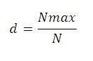
Where aj = abundance (proportion) of species j in sample, vj = indicator value and sj = pollution sensitivity of species j.

The performance of the indices depends on the values given to the constants s and v for each taxon and the values of the index ranges from 1 to an upper limit equal to the highest value of s. Each diatom species used in the calculation/equation is assigned two values; the first value reflects the tolerance or affinity of the diatom to a certain water quality (good or bad) while the second value indicates how strong (or weak) the relationship is. Abundance and weighted average were computed. This would indicate how many of the particular diatoms in the sample occur in relation to the total number counted.

Table 2 : Diatom Indices