2.1 Study Area
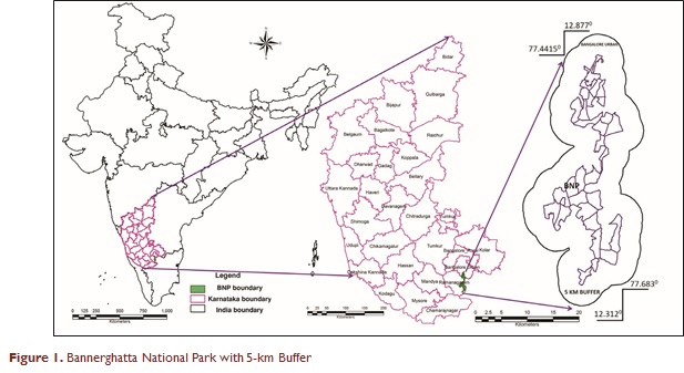
BNP encompasses an area of 260 sq.km, comprising of 13 reserve forests spread over the districts of Bangalore urban, Bangalore rural and Ramanagara districts; it was declared as a national park in 1974 (Figure 1). BNP is located in the south-east tip of Western Ghats with biological, social, hydrological and ecological significance and forms a vital conduit of the animal movement path. Forests in BNP have been aiding Bangalore’s climate and necessities through carbon sequestration, the mitigation of human-animal conflicts, the repository of diverse flora and fauna, recreation and pollination services as well as micro-climate moderation. BNP is one of the oldest prime habitats of Asian elephants, supporting a population of 100–150 and a migratory population of a large number, about 200–300, from the adjoining Tali Reserve Forest and Cauvery Wildlife Sanctuary; it acts as a terminal point for Eastern Ghats and Western Ghats. BNP, being part of the Western Ghats (one among 35 global biodiversity hotspots), is known for high species diversity, structural organization, spatial heterogeneity and adaptation to dry climate, moisture stress and irregular rainfall. The average temperature ranges from 22°C to 35°C and the annual monsoon rainfall varies from 625 mm to 1,607 mm, from June to mid-November, from south-west and north-east monsoons. The terrain represents undulating land with broken chains of bolder, strewn hillocks and hills of rocky outcrop and water courses. The forest types cover moist deciduous forests, dry deciduous forests, thorny scrub and grasslands with rich flora and fauna. The cropping pattern of BNP and its environs (5 km) is very much a modern system of agriculture due to its proximity with Bangalore. The farmers grow commercial crops such as banana, coconut, vegetables, sugarcane, mulberry and various flowers. Streams such as Suvarnamukhi, Hebballa, Suddahalla, Jakkanahalla Muthyalammamadu holé, Rayathmala holé and Anthragange halla are present in the region which support major crops. Floral diversity includes Cissampelos pareira, Decalepis hamiltonii, Cardiospermum halicacabum, Gloriosa superba, Cassia fistula, Wrightia sp., Holarrhena pubescens, Aegle marmelos, Shorea roxburghii, Phyllanthus emblica and so on
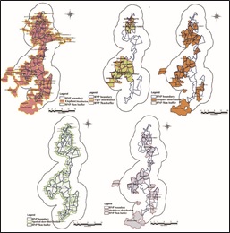
They are highly valued medicinal plants, many of them rare or endangered and traded in high volumes. A total of 218 plants belonging to 60 families were recorded during the survey. Among these, trees (81 species) and herbs (88 species) had the highest number of species, followed by shrubs (34 species) and climbers (15 species). About 80 species of birds were recorded during the survey, which include migratory birds of winter such as Golden Oriole, Forest Wagtail, Rosy Starling, Booted Warbler, Greenish Warbler, Ultramarine Flycatcher, Lesser Spotted Eagle, Pallid Harrier and Wire Tailed Swallow and so on. The presence of these bird species highlights rich habitats with supporting niche. The distribution of various faunal species such as elephants, tigers, leopards, spotted deer and sloth bears is shown in Figure 2. However, an increase in anthropogenic activities with the increase in human habitation and the expansion of agricultural and horticultural activities have threatened the survival of these fragile ecosystems. The anthropogenic activities include the unsustainable exploitation of forest resources, the encroachment of forests, stone quarrying, sand mining, domestic livestock grazing and unplanned urbanization; they have become a major threat to the conservation of forests and its resources.

Figure 2. The Distribution of Various Faunal Species in Bannerghatta National Park

2.2 Land Use Land Cover Analysis
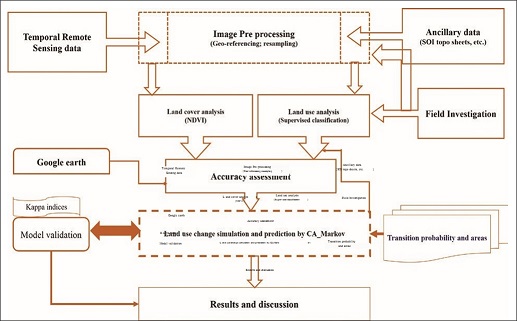
Landscape dynamics in the BNP region is assessed with the help of temporal spatial data acquired through spaceborne sensors (RS data), ancillary data (collateral data compiled from government agencies) and primary data compiled through field investigations (ground control points and training data—polygons of land uses with attribute information). Figure 3 outlines the protocol followed to analyse land uses from the spatial data. RS data used in the study are Landsat MSS (1973), TM (1989, 1999), Landsat ETM + (2009), downloaded from the public domain (http://landsat.org), IRS p6L4X (2015) (http://nrsc. gov.in) and the online Google Earth portal (http://earth. google.com). Ancillary data were used to assist the interpretation of different land use types from RS data. Topographic maps provided ground control points to rectify remotely sensed data and scanned paper maps (topographic maps) and assigned the UTM (zone 43 N) projection system. The Survey of India (SOI) topographic maps (scale: 1:50000 and 1:250000) and vegetation maps of South India (scale: 1:250000) developed by the French Institute (1986) were digitized to identify various forest cover types and for temporal analyses to understand vegetation changes. Field data (ground control points and training data) were collected with the help of pre-calibrated GPS (global positioning system, Garmin GPS unit). Ground control points were used for the geometric rectification of RS data. The training data were used for the classification of RS data (land use analysis) based on supervised classification approaches through the Gaussian maximum likelihood (GML) algorithm. Land cover analysis was conducted to understand the extent of vegetation cover using the normalized difference vegetation index (NDVI) as per Equation (1). NDVI, also known as a greenness index, values ranges between −1 to and +1 and helps in delineating vegetation cover.
NDVI = (NIR − R) / (NIR + R) (1)
Land use analyses using remote sensing data involved (a) the generation of false colour composite (FCC) of RS data (bands: green, red and Near Infrared [NIR]). This composite image helped in locating heterogeneous patches in the landscape, (b) the selection of training polygons covering 15 per cent of the study area (polygons are uniformly distributed over the entire study area), (c) loading these training polygon coordinates into the pre-calibrated GPS and (d) the collection of the corresponding attribute data (land use types) for these polygons from the field. GPS helped in locating respective training polygons in the field, (e) supplementing this information with Google Earth and (f) a total of 60 per cent of the training data were used for classification, while the balance were used for accuracy assessments (Bharath et al., 2013; Congalton, 1991; Jensen, 2005; Ramachandra, Bharath, & Sanna, 2012) by error matrix and kappa statistics (Anderson, Hardy, Roach, & Witmer, 1976; Liu, Frazier, & Kumar, 2007). Land use analysis was conducted using a supervised classification technique based on the GML algorithm with training data (collected from the field using GPS). Gaussian maximum likelihood (GML) is a widely used statistical classification method which assigns a given pixel to a specific class based on conditional probability. The likelihood for a given pixel with a spectral value to be assigned to a class is determined using Bayes’ theorem and the decision rule calculated by natural logarithm or ‘discriminant function’ (Lillesand, Kiefer, & Chipman, 2014). Geographical Resources Analysis Support System (GRASS GIS, http://ces.iisc. ernet.in/grass), a free and open-source software with robust support for processing both vector and raster data, was used to analyse RS data through available multi-temporal ‘ground truth’ information (http://ces.iisc.ernet.in/grass).

Figure 3. Method Followed in the Analysis

2.3 Modelling Spatial Patterns of Transitions
Land use analyses provided spatial patterns at the temporal scale and the Markovian process aided to generate the transition probability map and area matrix based on the probability distribution of the current cell state that was assumed to only depend on the current state (Equations [2] and [3]). The land use maps of 1999–2015 were reclassified into five categories for effective visualization as explained in Table 1. The original transition probability matrix (denoted as P) of land use types can be obtained from two former land use maps. Cellular automata was used to obtain a spatial context and distribution map based on Markov’s transitional probability and area by combining multicriteria land allocation to predict land cover change over time. The water category was considered a constraint (assuming that this category continues to exist). The transition rules were made considering the possibility of forests transforming to other land uses, agriculture and built-up transform forests. The rate of transitions was based on past land use changes and current trends, ascertained through field investigations. Also, the city’s developmental plans of 2015 (available at http://bbmp.gov.in/revisedmaster-plan) and 2031 (http://www.bmrda.kar.nic.in/rsp_ report.pdf) have been used in the analysis. The proposed housing and industrial layouts were digitized and considered as the future growth poles to simulate the possible land use transitions. The net neighbourhood influences were determined by the 5 × 5 contiguity filter which explains past land use changes and used to simulate future changes. Land use predictions of 2015 were made using CA coupled with Markov chains based on the transitional probability generated for 1999–2009. The validation of predicted land use was done by comparing it with reference land use of 2015 (actual) through the computation of kappa index (for location and quantity). This helped in the visualization of likely land uses in 2027, considering 6-year time intervals.
P N( ) = P N( − 1) × Pij (2)
where P(N) is state probability at any time and P(N − 1) is preliminary state probability.
Transition area matrix can be obtained by,
where Pij is the sum of areas from the ith land use category to the jth category in the years from start point to target simulation periods and n is the number of land use types. The transition area matrix must meet the following conditions (Equations (4) and (5)):
i. 0 ≤ Pij ≤ 1 (4)
n ii. ∑Pij = 1 (5)
i j, =0

Table 1. Land Use Classes Considered for the Analysis