Data and methods

The study includes assessment of energy at supply side and demand side and is detailed in Figure 3. The supply side includes assessment of regional solar energy availability, spatial extent of rooftop (individual households) and waste land (in the respective villages). The demand side includes estimation of domestic electricity consumption in households and irrigation as well as the extent of rooftop/land area required for installing PV based systems to meet the decentralised demand.

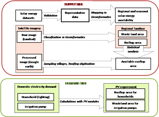Figure 3: Flow chart of the study

4.1 Assessment of solar energy potential 

Village-wise solar energy availability in Uttara Kannada was assessed using satellite-based high resolution global insolation data derived on prudent models. Two datasets collectedwere:

1. Surface Meteorology and Solar Energy (SSE) 1°x1° (~100 X 100 km) spatial resolution global horizontal insolation (GHI) data provided by National Aeronautics and Space Administration (NASA) based on satellite measurements of 22 years (July 1983 to June 2005) (Surface Meteorology and Solar Energy Release 6.0 Methodology, NASA, 2012);
2. Higher spatial resolution 0.1° X 0.1° (~ 10 X 10 km) GHI data furnished by the National Renewable Energy Laboratory (NREL) based on satellite measurements of 7 years (January 2002 to December 2008) (NREL GHI data furnished by National Renewable energy Laboratory, 2010). These were compared and validated with long term surface GHI measurements based interpolation model for the region.Higher resolution NREL GHI data were used to study the seasonal availability and variability of village-wise solar energy in Uttara Kannada. Seasonal solar maps were generated using Geographic Information Systems (GIS) tools (Ramachandra, Krishnadas Gautham and Jain Rishab, 2012a, P: 8).

4.2 Estimation of Builtup and Rooftop area (Digitization of rooftop area)

4.2.1 Estimation of Builtup area:
Multispectral data acquired through IRS (Indian Remote Sensing) P6 satellite of 5.8 m resolution was used to estimate the extent of human habitations. Remote sensing data were analysed through standard protocols involving geometric correction, image classification through Gaussian maximum likelihood classifier. The remote sensing data obtained were geo-referenced, rectified and cropped pertaining to the study area. Geo-registration of remote sensing data (IRS P6) has been done using ground control points collected from the field using pre calibrated GPS (Global Positioning System) and also from known points (such as road intersections, etc.) collected from geo-referenced topographic maps published by the Survey of India (1:50000, 1:250000). Analysis of remote sensing data (Ramachandra, Aithal and Durgappa, 2012, P328-333) involved i) generation of False Colour Composite (FCC) of remote sensing data (bands – green, red and NIR). This helped in locating heterogeneous patches in the landscape ii) selection of training polygons (these correspond to heterogeneous patches in FCC) covering 15% of the study area and uniformly distributed over the entire study area, iii) loading these training polygons co-ordinates into pre-calibrated GPS, vi) collection of the corresponding attribute data (land use types) for these polygons from the field. GPS helped in locating respective training polygons in the field, iv) supplementing this information with Google Earth  v) 60% of the training data has been used for  classification, while the balance is used for validation or accuracy assessment.

Land use analysis was carried out through open source program GRASS - Geographic Resource Analysis Support System (http://grass.fbk.eu/) using supervised pattern classifier - Gaussian maximum likelihood algorithm using probability and cost functions (Ramachandra, Aithal and Durgappa, 2012, P328-333). Accuracy assessment to evaluate the performance of  classifiers, was done  with the help of field data by testing the statistical significance of a difference,  computation of kappa coefficients and  proportion of correctly allocated cases.   Statistical assessment of classifier performance based on the performance of spectral classification considering reference pixels is done which include computation of kappa (κ) statistics and overall (producer's and user's) accuracies. Application of  maximum likelihood classification method resulted in accuracy of 88%. Remote sensing data analysis provided i) area under vegetation (forests, grass lands.), ii) built up (buildings, roads or any paved surface, iii) water bodies (lakes/tanks, rivers, reservoirs), iv) others (open area such as play grounds, quarry regions, etc.).

4.2.2 Estimation of the spatial extent of rooftops:
Regional rooftop area availability for harvesting solar energy was calculated using remote sensing data through geo-informatics and statistical tools. Villages representing different agro-climatic zones of Uttara Kannada were randomly chosen and rooftop areas were mapped by manual digitisation of high resolution Google Earth satellite data (http://googleearth.com) with the support of geo-informatics tools (Ordonez et al., 2010, P: 2124, Ramachandra, 2007, P: 108). Roof types in towns and other urban areas were similar in most of the zones, one random sample was manually digitised for estimating the spatial extent of rooftops. The built-up areas for randomly sampled regions and manually digitized total rooftop areas were investigated using statistical tools. Total rooftop areas were extrapolated for other regions based on two different methods:

1. Method 1– Census based: Ratio of total rooftop area to number of households (census) in sampled regions provided average rooftop area per household  for respective agro-climatic zones i. These ratios were used to derive total rooftop areas  in other regions based on number of households  from the census, as shown in equation 1.  value for towns were taken as same in all agro-climatic zones.

 --------------- (1)
where, Ri is the total rooftop area of households in i^th agro-climatic zone in m²
Hi is the number of households in ith agro-climatic zone 

2. Method 2–based on Land Use Land Cover (LULC): Signature separation corresponding to LU (Land Use) classes is done using Transformed Divergence (TD) matrix and Bhattacharya distance. Accuracy assessment is done using error matrix in order to get most precise results (Ramachandra, Joshi and Kumar Uttam, 2012, P: 3). Ratios of total rooftop areas to built-up areas in sampled regions were averaged  over different agroclimatic zones i. Ratios with large deviations were removed due to possibility of misclassification. The average ratio values for respective zones were used to derive total rooftop areas  in other villages, as shown in equation 2.

--------------- (2)
where, Bi is the total-built up area in i^th agro-climatic zone 

4.3 Regional domestic electricity demand:

Taluk wise electricity consumption data were collected from the respective government agencies. Apart from this, stratified random sampling of 1,700 households representing all agro-climatic zones yielded energy requirement per household. Based on this data, monthly electricity usage (in kWh) for household for purposes like lighting, heating etc, and irrigation pump sets were computed (Ramachandra, Joshi, et al., 2000, P: 825).

4.4 PV requirement to meet regional electricity demand: Electricity generation from PV was calculated based on the equation 3.  The theoretical energy output from a PV cell,

----------------- (3)
where, G is the Global Horizontal Insolation (kWh/m²),
A is the area of the PV panel,
P is the rated power output,
Istc is the insolation at standard test conditions and η is the efficiency.

Actual energy output considering the quality factor,
------------------- (4)    
where, Q is the quality factor of a PV module. Hence wattage of PV to be installed is found by
  --------------------- (5)
Area required to meet the demand is,
  ----------------------- (6)

The built-up areas for randomly sampled villages and manually digitized roof-top areas were compared using parametric tests (paired t-test) (Sampling Techniques, C.E.C.S.A., 1975). Ratio of total rooftop area to number of households (census) in sampled villages provided rooftop area per household for respective agro climatic zones. These ratios were used to derive rooftop areas in other villages based on number of households. Percentage share of manually digitized rooftop area in the total classified built-up area for sampled town was estimated. This factor was used for all other town panchayats and municipalities to estimate rooftop areas available. Computed rooftop area is assumed to be available for installing solar energy applications like photovoltaic panels, water heaters, etc. to meet the lighting and water heating requirement of respective houses.
Figure 4 depicts the digitized rooftops in Lakolli village of Mundgod Taluk in Uttara Kannada. The polygons of exposed (available) rooftops in a village are manually digitised using Google Earth. Rooftops in 30 random regions (including one town) spread across four agro-climatic zones of Uttara Kannada were similarly digitised. Rooftop area per household  was calculated for the sampled villages and averaged over each agro-climatic zone respectively. These are given in Table 1 and details of villages/towns in Appendix I.

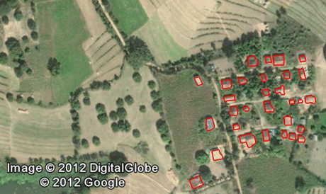Figure 4: Rooftop digitisation in Lakolli village of Mundgodtaluk,Uttara Kannada

Table 1: Average values of R/H and R/B ratios for different agro-climatic zones

APPENDIX I:
Sampled regions