|
Fusion of Multisensor Data: Review and Comparative Analysis |  |
 |
 |
 |
 |
 |
 |
 |
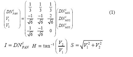
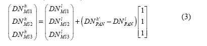
Image Fusion Techniques RS data are radiometrically and geometrically corrected (at pixel level) and georegistered considering the topographic undulations. For all methods discussed here, it is assumed that LR MS images are upsampled to the size of HR PAN image. Intensity-Hue-Saturation (IHS) In RGB – IHS algorithm, the LR MS data (DNlMS1, DNlMS2, DNlMS3) are transformed to the IHS (Intensity, Hue, Saturation) color space (equation 1) which separates the colour aspects in its average brightness (intensity). This corresponds to the surface roughness, its dominant wavelength contribution (hue) and its purity (saturation) [5]. V1 and V2 are the intermediate variables. I is replaced with HR image – DNh’PAN and is contrast stretched to match the original PAN image. The fused images of HR are obtained by performing an inverse transformation (equation 2).
Since the forward and backward transformations are linear, replacing V1 and V2 in equation (2) by V1 and V2 from (1) yields the mathematical model (equation 3) where DNlPAN = (1/3) (DNlMS1 + DNlMS2 + DNlMS3) and DNh’PAN is DNhPAN, stretched to have same mean variance as DNlPAN.
Brovey Transform (BT) BT is based on the chromaticity transform with a limitation that only three bands are involved [6]. It normalises the three MS bands used for RGB display and to multiply the result by any other desired data to add the intensity or brightness component to the image (equation 4) where DNlPAN = (1/3) (DNlMS1 + DNlMS2 + DNlMS3). 
High pass filtering (HPF) The high spatial resolution image is filtered with a small high-pass (HP) filter or taking the original HR PAN image and subtracting the LR PAN image, which is the low-pass (LP) filtered HR PAN image resulting in the high frequency part of the data which is related to the spatial information. This is pixel wise added to the LR bands. It preserves a high percentage of the spectral characteristics, since the spatial information is associated with the high-frequency information of the HR MS images, which is from the HR PAN image, and the spectral information is associated with the low-frequency information of the HR MS images, which is from the LR MS images (equation 5) [6].
where DNlPAN = DNhPAN * h0 and h0 is a LP filter (average or smoothing filter). High pass modulation (HPM) This transfers the high frequency information of PAN to LR MS data, with modulation coefficients, which equal the ratio between the LR MS images and the LR PAN image [6] where DNlPAN = DNhPAN * h0 and h0 is the same LP filter as used in the HPF method.
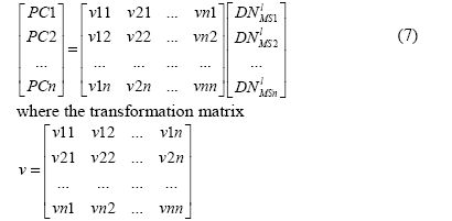
Principal Component Analysis (PCA) This transforms multivariate data into a data set of new un-correlated linear combinations of the original variables. It follows the idea similar to the IHS, of increasing the spatial resolution of MS images by introducing a HR PAN image, with the main advantage that an arbitrary number of bands can be used. The channel which will replace PC1 is stretched to the variance and average of PC1. The HR image replaces PC1 since it contains the information which is common to all bands while the spectral information is unique for each band. PC1 accounts for maximum variance which can maximise the effect of the HR data in the fused image. Finally, HR MS images are determined by performing the inverse PCA transform. The transformation matrix v contains the eigenvectors, ordered with respect to their eigenvalues. It is orthogonal and determined either from the covariance or correlation matrix of the input LR MS images [6].
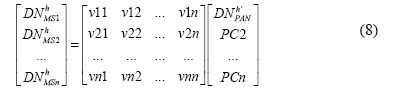
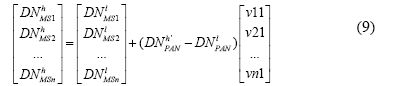
Similar to IHS method, equation 7 and 8 can be merged as follows:
where DNlPAN = PC1 and DNh’PAN is DNlPAN, stretched to have same mean and variance as PC1. Fourier transformation (FT) FT or filter fusion transfers the high spatial frequency content of the HR image to the MS imagery by combining the LP filter version of the duplicated LR MS image and a HP filter version of the more highly resolved PAN [7]. This preserves a high percentage of the spectral characteristic, since the spectral information is associated with the low spatial frequencies of the MS imagery. The spatial resolution data is extracted by HP filtering the more highly resolved PAN band. The cut-off frequencies of the filters have to be chosen in such a way that the included data does not influence the spectra of the opposite data. A sensible value is the Nyquist frequency of the MS imagery. The fusion process is shown in equation (10) where FT denotes the Fourier transformation.
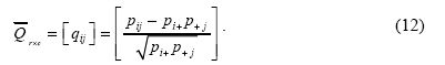
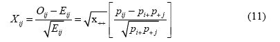
The usage of the spatial frequency domain is convenient for the filter design and allows a faster computation for large imagery. After fusing both filtered spectra, the inverse Fourier transform (FT-1) leads back into the image domain. The limitation of the approach is the introduction of false edges if the LR MS bands and the HR PAN exhibit a weak correlation. Correspondence Analysis (CA) Here, the data table (X) is transformed into a table of contributions of the Pearson chi-square statistic [1]. First, pixel (Xij) values are converted to proportions (Pij) by dividing each pixel (Xij) value by the sum (x++) of all pixels in data set. The result is a new data set of proportions (table Q), and the size is r x c. Row weight pi+ is equal to xi+/x++, where xi+ is the sum of values in row i. Vector [p+j] is of size c. The Pearson chi-square statistic, χ2p, is a sum of squared χij values computed for every cell ‘ij’ of the contingency table:
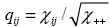
If we use qij values instead of Xij values, so that
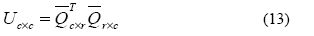
After this point, the calculation of eigenvalues and the eigenvectors is similar to the PCA methods. Matrix U produced by
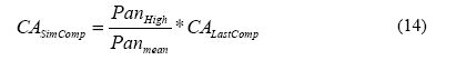
is similar to the covariance matrix of PCA. MS data are then transformed into the component space using the matrix of eigenvectors. A difference between CA and PCA fusion is the substitution of the last component with the high spatial resolution imagery as opposed to the substitution of the first component in the PCA. Two methods can be used in this part of the CA fusion process. The first is the substitution of the last component with PAN, which is stretched to have same range and variance with the last CA component. Second is the inclusion of details from the PAN band into the last component. Spatial details can be represented as the ratios of pixel values at the lower resolutions of the same imagery and can be included into the last component by
|


 , eigenvalues will be smaller than or equal to 1 which is more convenient. We used the qij values to form matrix
  which is