|
DATA, MODELS AND METHODS
1. Surface wind measurements
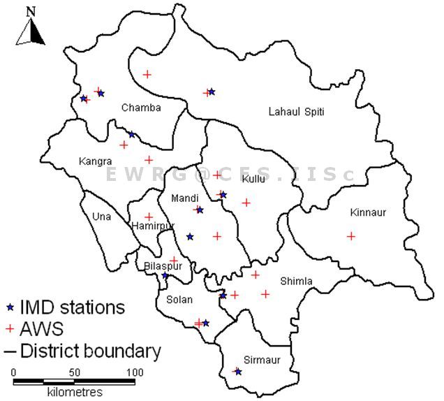
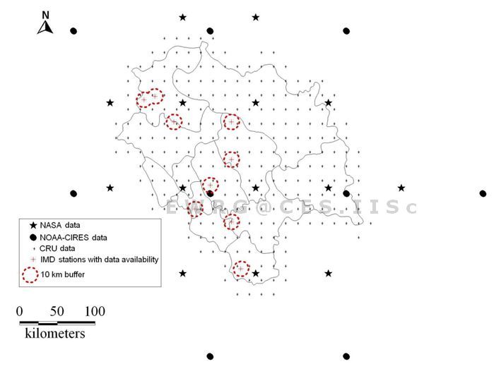
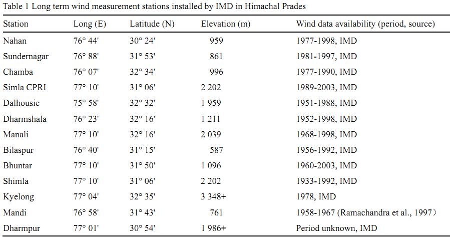
Long term wind characteristicsin Himachal Pradesh were recorded at 13 meteorological stations (Figure 2) of the India Meteorological Department (IMD). Table 1 lists the IMD stations and periods of wind measurement exercises. Wind speed measurement heights varied from 1.7 m (Dalhousie), 5 m (Manali), 7 m (Dharmshala), 9.7 m (Bilaspur) to 26 m (Kyelong) and 26.5 m (Shimla).
Out of 13, IMD provided surface wind data for 10 stations (Bilaspur, Sundernagar, Nahan, Chamba, Bhuntar, Dharmshala, Dalhousie, Manali, Simla CPRI and Shimla) recorded for different durations (Table 1). Wind speed at Mandi was obtained from a literature on wind climatology in India (Mani and Mooley, 1983). The measured data included: 1) synoptic hour values (local time 8:30 and 17:30 hrs); 2) daily averages for durations between synoptic hours and; 3) monthly averages (not available for Mandi) of wind speeds. Daily averages of wind speeds were obtained by averaging the mean for two 12 hour periods starting from 17:30 hrs, capturing the diurnal variations of the wind. Wind measurements were standardized to 10m using power law equation (1) as per World Meteorological Organization (WMO) norm (Ramachandra et al., 1997).
 (1) (1)
where Vo is the measured wind speed, V is the standardized wind speed, Ho is the measured height, H is the desired height (10m) and α is the power law index. Here α is a measure of roughness due to frictional and impact forces on the ground surface which varies according to terrain, time and seasons. The value of α calculated for most of the regions representing the Himalayan terrain are well above 0.40 based on long term observations and calculations (Mani and Mooley, 1983). In order to minimize extrapolation errors we considered the least value of 0.40 for Himachal Pradesh. The wind measurement heights in Himachal Pradesh were standardized using power law equation with α as 0.4.
Topography of Himachal Pradesh renders enormous variation to the micro–climate, wind speeds and direction, adding to complexity of wind resource assessment in the region. The available IMD surface wind data were characterized by large gaps and non–standard measurement heights. In addition, these stations were not representative of the diverse agroclimatic zones and particularly unavailable for the high elevation zone (>3500 m) of Himachal Pradesh (Figure 2). Capturing the wind regime of its complex terrain using these data cannot be a desirable option. Recently, IMD has deployed Automatic Weather Stations (AWS) at 22 locations in Himachal Pradesh (Figure 2) at 2 m heights above the ground (AWS, 2012). However, according to the communication from IMD, AWS based wind data were available merely for 3 stations (Bilaspur, Una and Udaipur) for the year 2011. Hence, we explored long term global wind datasets synthesised based on prudent models appropriate for the study area.
Table I: Long term wind measurement stationsinstalled by IMD in Himachal Pradesh
| Station |
Long
(E) |
Lat
(N) |
Elevation
(m) |
Wind data availability
(period, source) |
| Nahan |
76° 44' |
30° 24' |
959 |
1977-1998, IMD |
| Sundernagar |
76° 88' |
31° 53' |
861 |
1981-1997, IMD |
| Chamba |
76° 07' |
32° 34' |
996 |
1977-1990, IMD |
| Simla CPRI |
77° 10' |
31° 06' |
2202 |
1989-2003, IMD |
| Dalhousie |
75° 58' |
32° 32' |
1959 |
1951-1988, IMD |
| Dharmshala |
76° 23' |
32° 16' |
1211 |
1952-1998, IMD |
| Manali |
77° 10' |
32° 16' |
2039 |
1968-1998, IMD |
| Bilaspur |
76° 40' |
31° 15' |
587 |
1956-1992, IMD |
| Bhuntar |
77° 10' |
31° 50' |
1096 |
1960-2003, IMD |
| Shimla |
77° 10' |
31° 06' |
2202 |
1933-1992, IMD |
| Kyelong |
77° 04' |
32° 35' |
3348+ |
1978, IMD |
| Mandi |
76° 58' |
31° 43' |
761 |
1958-1967, [6] |
| Dharmpur |
77° 01' |
30° 54' |
1986+ |
Period unknown, IMD |
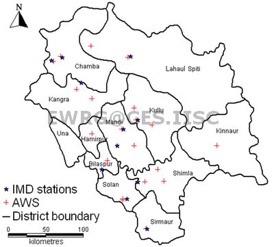
Figure 2: Total wind stations in Himachal Pradesh
2. Available synthesised wind data
2.1. NASA SSE
The National Aeronautics and Space Administration (NASA) Langley Research Center Surface Meteorology and Solar Energy (SSE) meteorological datasets were derived from a variety of earth-observing satellites. Particularly, NASA-SSE 10-year (1983–1993) monthly average wind speeds at 1oX1o spatial resolution for different heights above the earth’s surface weredeveloped based on a Global Circulation Model (GCM) applied on the outputs from Goddard Earth Observing System (GEOS). It is known that, vegetation and canopy reduces near-surface wind speeds variably. Hence, based on parameterizations developed from observations in Canada, Scandinavia, Africa, and South America, NASA synthesised wind speeds for 17 surface/vegetation types at different heights (Takacs et al., 1996; NASA 2012).
According to NASA, synthesised SSE 10 m wind speed estimates for airport-like flat surfaceswere validated with 30-year average airport wind data over the globe furnished by the RET Screen project. This had an estimated uncertainty of Root Mean Square (RMS) 1.3 m/s that is 20-25% relative to mean monthly values (NASA, 2012). However, studies have shown that NASA-SSE wind data exceeds the 25% error margin even in plain regions when compared to surface measurements (Kumarand Prasad, 2010). The SSE modelers agree that 1°X1° spatial resolution wind data is not an accurate predictor of local conditions in regions with significant topographic variation. The NASA-SSE wind speed data were accessed at http://eosweb.larc.nasa.gov/sse/.
2.2. NOAA–CIRES
The National Oceanic and Atmospheric Administration (NOAA) and University of Colorado CIRES Climate Diagnostics Center synthesised comprehensive global atmospheric circulation dataset as per their Twentieth Century Reanalysis# project. NOAA–CIRES 20th Century Reanalysis Version 2 dataset provides estimates of global tropospheric and stratospheric variability since 1871 at six-hourly temporal resolution. These were derived based on surface and sea level pressure measurements. Monthly sea-surface temperatures and sea-ice distributions were considered as boundary conditions in an Ensemble Kalman Filter data assimilation with support of certain parameterizations andglobal numerical weather prediction (NWP) model (NOAA, 2012).The NWP model generates numerical simulations of the global atmospheric state, which are reanalysed and stored. However, NWP data are generally used as input of models which generate low resolution grids so as to infer the near-surface wind field. This process, called downscaling, is performed using statistical and dynamical considerations (Aguera-Perez et al., 2012). Global wind speeds of 138 years (1871–2008) at 2oX2o spatial resolutionwere accessed at http://www.esrl.noaa.gov/psd/data/20thC_Rean/.
2.3. CRU
Climate Research Unit (CRU) at the University of East Anglia maintainsclimatic average datasets of meteorological variables. This includes wind speeds for the period of 1961–1990 compiled from different sources with inter and intra variable consistency checks to minimize data consolidation errors. The Gobal Land One–km Base Elevation Project (GLOBE) data of the National Geophysical Data Center (NGDC) were re–sampled to 10’X10’ (ten minute spatial resolution) elevation grids where every cell with more than 25% land surface (those below 25% being considered water bodies) represents the average elevation of 100–400 GLOBE elevation points. The climatic average of wind speeds measured at 2 to 20m anemometer heights (assumed to be standardized during collection) collated from 3950 global meteorological stations together with the information on latitude, longitude and elevation were interpolated based on a geo–statistical technique called thin plate smoothing splines. Elevation as a co–predictor considers topographic influence on the wind speed and proximity of a region to the measuring station improves the reliability of the interpolated data. During interpolation inconsistent data were removed appropriately. This technique was identified to be steadfast in situations of data sparseness or irregularity (New et al., 2002). The 10’X10’ spatial resolution wind speed data as climatic averages were available for all global regions (excluding Antarctica). Thesewere accessed at http://www.cru.uea.ac.uk/cru/data/hrg/tmc/.
3. Wind profiling
Synthesised wind speed data collected from NASA-SSE, NOAA-CIRES and CRU covering the study area of Himachal Pradesh grid-wise is represented in Figure 3 along with IMD surface measurement sites for which data were provided. Based on the spatial as well as ground (field visits) understanding of agroclimatic zones inHimachal Pradesh, 10 m surface/vegetation influenced wind speeds were collected from NASA-SSE for 14 grids (locations) at 1oX1o spatial resolution. These surface/vegetation types included: 1) rough glacial snow/ice (six locations above 3500 m); 2) needleleaf-evergreen trees (three locations within 1000-3500 m) and; 3) broadleaf-needleleaf trees (five locations below 1000 m). Similarly, 2oX2o coarse spatial resolution wind speeds for 9 grids and 10’X10’ high spatial resolution wind speeds for 266 grids were collected from NOAA-CIRES and CRU respectively (Figure 3). The collected wind speed data from NASA-SSE, NOAA-CIRES and CRU were interpolated using geospatial techniques to observe the annual wind speed regime over Himachal Pradesh. These data were validatedand cross-compared with available surface wind speed measurements using statistical methods to identify the most representative data for the study area. Regional variations of this wind data were re-validated with surface measurement in proximity by generating buffers of 10 km around the IMD sites. Monthly average wind speed values fromtherepresentative synthesiseddata were used to produce seasonal wind profiles for Himachal Pradesh. These seasonal wind variations were compared with surface measurements from IMD.
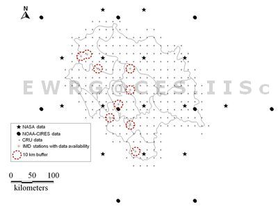
Figure 3: Synthesized as well as surface (IMD) wind speed locations for Himachal Pradesh
#Reanalysis is a scientific method for developing a comprehensive record of how weather and climate are changing over time wherein observations and a numerical model that simulates one or more aspects of the Earth system are combined objectively to generate a synthesized estimate of the state of the system (Reanalysis Intercomparison and Observations, 2012).
|
