METHODS
A. Maximum Likelihood classifier (MLC) – Supervised classification of the image was performed using MLC. MLC has become popular and widespread in RS because of its robustness [3–6]. It quantitatively evaluates both the variance and covariance of the category spectral response pattern [7] assuming the distribution of data points to be Gaussian [8] which is described by the mean vector and the covariance matrix. The statistical probability of a given pixel value being a member of a particular class is computed and the pixel is assigned to the most likely class (highest probability value). If the training data pertaining to different classes contain n samples and the samples in each class are i.i.d. (independent and identically distributed) random variables and further if we assume that the spectral classes for an image is represented by ωn, n=1,…, N, where N is the total number of classes, then probability density p(ωn|x) gives the likelihood that the pixel x belongs to class ωn where x is a column vector of the observed digital number of the pixels. It describes the pixel as a point in multispectral space (M-dimensional space, where M is the number of spectral bands). The maximum likelihood (ML) parameters are estimated from representative i.i.d. samples. Classification is performed according to

i.e., the pixel x belongs to class ωn if p(ωn|x) is largest. The ML decision rule is based on a normalised estimate of the probability density function (p.d.f.) of each class. The discriminant function, gln(x) for ωn in MLC is expressed as

where p(ωn) is the prior probability of ωn, p(x|ωn) is the p.d.f. for pixel vector x conditioned on ωn [6]. Pixel vector x is assigned to the class for which gln(x) is greatest. In an operational context, the logarithm form of (2) is used, and after the constants are eliminated, the discriminant function for ωn is stated as

where  is the variance-covariance matrix of ωn, μn is the mean vector of ωn. A pixel is assigned to the class with the lowest
  [6, 9-10]. For each LU class (agricultural land, human settlement / residential / commercial areas, roads, forest, plantation, waste land / open land and water bodies) training samples were collected representing approximately 10% of the study area. With these 10% known pixel labels from training data, the aim was to assign labels to all the remaining pixels in the image.
B. Forest fragmentation: Forest fragmentation is the process whereby a large, continuous area of forest is both reduced in area and divided into two or more fragments. The decline in the size of the forest and the increasing isolation between the two remnant patches of the forest has been the major cause of declining biodiversity [11-15]. The primary concern is direct loss of forest area, and all disturbed forests are subject to “edge effects” of one kind or another. Forest fragmentation is of additional concern, insofar as the edge effect is mitigated by the residual spatial pattern [16-19].
LU map indicate only the location and type of forest, and further analysis is needed to quantify the forest fragmentation. Total extent of forest and its occurrence as adjacent pixels, fixed-area windows surrounding each forest pixel is used for calculating type of fragmentation. The result is stored at the location of the centre pixel. Thus, a pixel value in the derived map refers to between-pixel fragmentation around the corresponding forest location. As an example [20], if Pf is the proportion of pixels in the window that are forested and Pff is the proportion of all adjacent (cardinal directions only) pixel pairs that include at least one forest pixel, for which both pixels are forested. Pff estimates the conditional probability that, given a pixel of forest, its neighbour is also forest. The six fragmentation model that identifies six fragmentation categories are: (1) interior, for which Pf = 1.0; (2), patch, Pf < 0.4; (3) transtitional, 0.4 < Pf < 0.6; (4) edge, Pf > 0.6 and Pf-Pff > 0; (5) perforated, Pf > 0.6 and Pf-Pff < 0, and (6) undetermined, Pf > 0.6 and Pf = Pff. When Pff is larger than Pf, the implication is that forest is clumped; the probability that an immediate neighbour is also forest is greater than the average probability of forest within the window. Conversely, when Pff is smaller than Pf, the implication is that whatever is non-forest is clumped. The difference (Pf-Pff) characterises a gradient from forest clumping (edge) to non-forest clumping (perforated). When Pff = Pf, the model cannot distinguish forest or non-forest clumping. The case of Pf = 1 (interior) represents a completely forested window for which Pff must be 1.
C. Support Vector Machine (SVM): SVM are supervised learning algorithms based on statistical learning theory, which are considered to be heuristic algorithms [21]. SVM map input vectors to a higher dimensional space where a maximal separating hyper plane is constructed. Two parallel hyper planes are constructed on each side of the hyper plane that separates the data. The separating hyper plane maximises the distance between the two parallel hyper planes. An assumption is made that the larger the margin or distance between these parallel hyper planes, the better the generalisation error of the classifier will be. The model produced by support vector classification only depends on a subset of the training data, because the cost function for building the model does not take into account training points that lie beyond the margin [21]. When it is not possible to define the hyper plane by linear equations, the data can be mapped into a higher dimensional space through some nonlinear mapping functions.
A free and open source software – openModeller [22] was used for predicting the probable landslide areas using SVM. openModeller (http://openmodeller.sourceforge.net/) includes facilities for reading landslide occurrence and environmental data, selection of environmental layers on which the model should be based, creating a fundamental niche model and projecting the model into an environmental scenario as shown in Fig. 1.
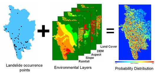
Fig. 1. Methodology used for landslide prediction in openModeller