 |
1 Energy & Wetlands Research Group, Centre for Ecological Sciences, 2 Centre for Sustainable Technologies (astra), 3 Centre for infrastructure, Sustainable Transportation and Urban Planning [CiSTUP] Indian Institute of Science, Bangalore – 560 012, India E-mail: cestvr@ces.iisc.ac.in |
MATERIALS AND METHOD
Table1. Materials used for the analysis
| DATA | Year | Purpose |
| Landsat Series Multispectral sensor (57.5m) | 1973 | Landcover and Land use analysis |
| Landsat Series Thematic mapper (28.5m) and Enhanced Thematic Mapper sensors | 1992, 1999, 2003, 2008, 2010 | Landcover and Land use analysis |
| Survey of India (SOI) toposheets of 1:50000 and 1:250000 scales | To Generate boundary and Base layer maps. |
a. Analysis flow
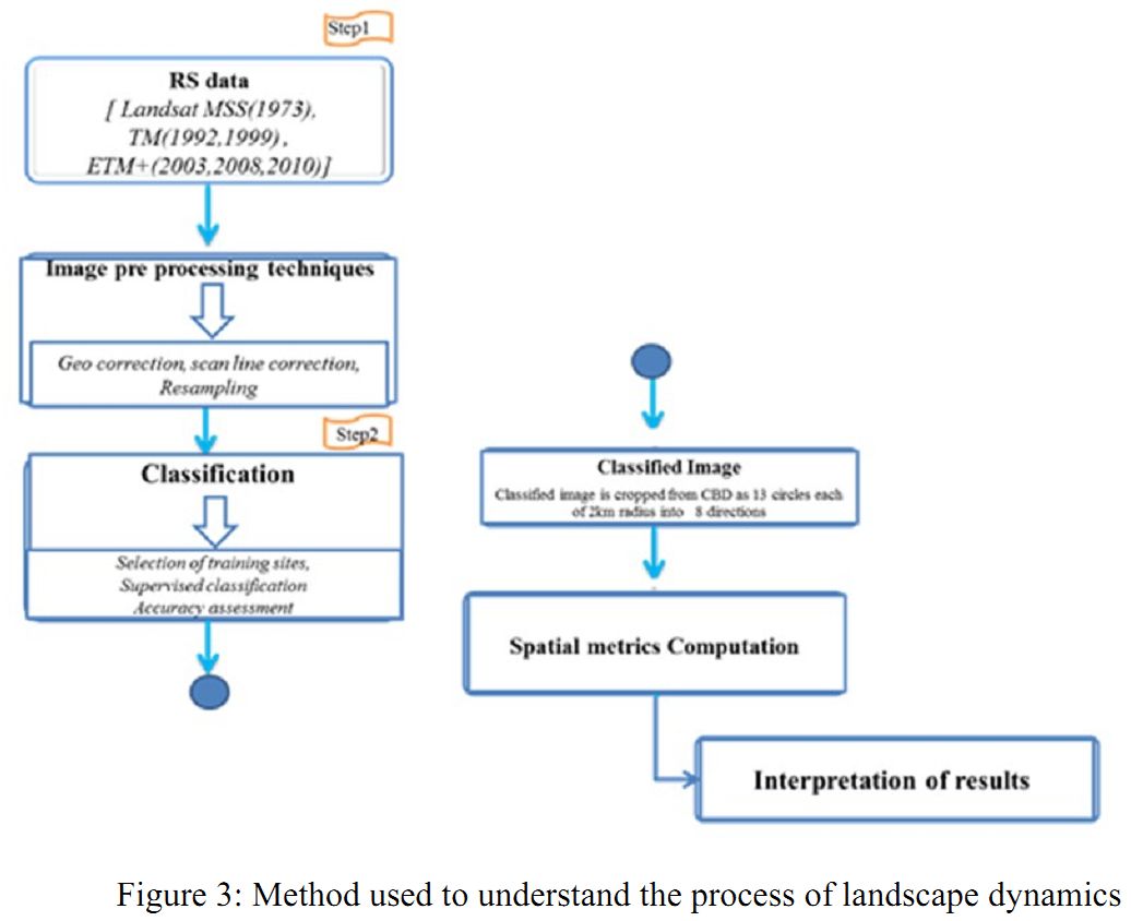
Figure 3: Method used to understand the process of landscape dynamics
Figure 3 illustrates the techniques followed in the analysis. Digital Remote sensing data were subjected to preprocessing to remove spectral and spatial biases. The data was geocorrected using GCPs (ground control points) and scan line correction especially for ETM+ data (SLC-off). The data is resampled to 30 m using nearest neighborhood algorithm, in order to maintain a common resolution across all the data sets.
The data was classified into four land use categories- urban, vegetation, water bodies and others with the help of training data using supervised classifier – Gaussian maximum likelihood. This preserves the basic land cover characteristics through statistical classification techniques using a number of well-distributed training pixels. GRASS (Geographical Analysis Support System) a free and open source software having robust support of processing both vector and raster files has been used for this analysis.Spectral classification inaccuracies are measured by a set of reference pixels. Based on the reference pixels, confusion matrix, kappa (κ) statistics and producer's and user's accuracies were computed. Accuracy assessment and kappa statistics are included in table 3. These accuracies relate solely to the performance of spectral classification.
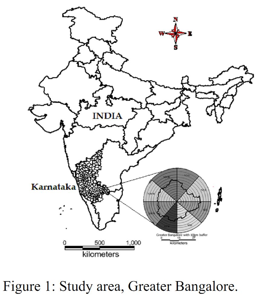
In step 2, to assess the spatio-temporal pattern of urban growth from the central business district(CBD) the classified image is divided into 13 circles in 8 directions (figure 1)with their origin from the ‘city center(CBD)’. The Shannon entropy &spatial metrics are calculated &analysed using fragstat for all images in 8 directions & 13 circles.
b. Analysis of urban sprawl (Shannon’s Entropy):
Shannon’s entropy (Yeh & Li, 2001; Sudhira et al, 2004) is used to measure the extent of urban sprawl with remote sensing data. Shannon’s entropy was calculated across all the directions considering each direction as an individual spatial unitis computed to detect the urban sprawl phenomenon given by the equation
 ..................... 1
Where, Pi is the Proportion of the variable in the ith zone & n the total number of zones. This value ranges from 0 to log n, indicating very compact distribution for values closer to 0. The values closer to log n indicates that the distribution is much dispersed. Larger value (close to log n) indicates fragmented growth indicative of sprawl.
c. Computation of Landscape metrics:
The gradient based approach is adopted to explain the spatial variation of urbanization (from the core region to the periphery). Landscape metrics were computed for each circle (region) in each direction to understand the spatio-temporal pattern of the landscape dynamics at local levels due to the urbanization process.
Table 2 lists the spatial metrics that have been computed to reflect the landscape’s spatial and temporal changes (Lausch & Herzog 2002). Thesemetrics are grouped into the five categoriesPatch area metrics, Edge/border metrics, Shape metrics, Compactness / contagion / dispersion metrics,
Table 2: Landscape metrics with significance
| Sl No | Indicators | Formula | Range | Significance/ Description | |||
| Category : Patch area metrics | |||||||
| 1 | Built up (Total Land Area) | ------ | >0 | Total built-up land (in ha) | |||
| 2 | Built up (Percentage of landscape ) |  A built-up = total built-up area A= total landscape area |
0<BP≤100 | It represents the percentage of built-up in the total landscape area. | |||
| 3 | Largest Patch |  ai = area (m2) of patch i A= total landscape area |
0 ≤ LPI≤1 | LPI = 0 when largest patch of the patch type becomes increasingly smaller. LPI = 1 when the entire landscape consists of a single patch of, when largest patch comprise 100% of the landscape. |
|||
| 4 | Mean patch size MPS |
 i=ith patch a=area of patch i n=total number of patches |
MPS>0, without limit | MPS is widely used to describe landscape structure. MPS is a measure of subdivision of the class or landscape. Mean patch size index on a raster map calculated, using a 4 neighbouring algorithm. | |||
| 5 | Number of Urban Patches |
NPU = n NP equals the number of patches in the landscape. |
NPU>0, without limit. | It is a fragmentation Index. Higher the value more the fragmentation | |||
| 6 | Patch density |
f(sample area) = (Patch Number/Area) * 1000000 | PD>0, without limit | Calculates patch density index on a raster map, using a 4 neighbor algorithm. Patch density increases with a greater number of patches within a reference area. | |||
| Category : Shape metrics | |||||||
| 7 | NLSI (Normalized Landscape Shape Index) |
 Where siand pi are the area and perimeter of patch i, and N is the total number of patches. |
0≤NLSI<1 | NLSI = 0 when the landscape consists of single square or maximally compact almost square, it increases when the patch types becomes increasingly disaggregated and is 1 when the patch type is maximally disaggregated | |||
| 8 | Mean Shape index MSI |
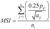 pij is the perimeter of patch i of type j. aij is the area of patch i of type j. ni is the total number of patches. |
MSI ≥ 1, without limit | Explains Shape Complexity. MSI is equal to 1 when all patches are circular (for polygons) or square (for raster (grids)) and it increases with increasing patch shape irregularity |
|||
| Category: Compactness/ contagion / dispersion metrics | |||||||
| 9 | Clumpiness | 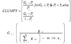 gii = number of like adjacencies (joins) between pixels of patch type (class) I based on the double-count method. gik =number of adjacencies (joins) between pixels of patch types (classes) i and k based on the double-count method. min-ei =minimum perimeter (in number of cell surfaces) of patch type (class)i for a maximally clumped class. Pi =proportion of the landscape occupied by patch type (class) i. |
-1≤ CLUMPY ≤1 | It equals 0 when the patches are distributed randomly, and approaches 1 when the patch type is maximally aggregated. | |||
| 10 | Aggregation index | 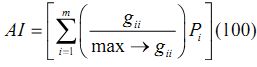 gii =number of like adjacencies (joins) between pixels of patch type (class) i based on the single count method. max-gii = maximum number of like adjacencies (joins) between pixels of patch type class i based on single count method. Pi = proportion of landscape comprised of patch type (class) i. |
1≤AI≤100 | AI equals 1 when the patches are maximally disaggregated and equals 100 when the patches are maximally aggregated into a single compact patch. Aggregation corresponds to the clustering of patches to form patches of a larger size. | |||
| Category : Open Space metrics | |||||||
| 11 | Ratio of open space (ROS) |
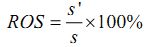 Where s is the summarization area of all “holes” inside the extracted urban area, s is summarization area of all patches |
It is represented as percentage. | The ratio, in a development, of open space to developed land. | |||
| * Corresponding Author : | |
| Dr. T.V. Ramachandra Energy & Wetlands Research Group, Centre for Ecological Sciences, Indian Institute of Science, Bangalore – 560 012, INDIA. Tel : 91-80-23600985 / 22932506 / 22933099, Fax : 91-80-23601428 / 23600085 / 23600683 [CES-TVR] E-mail : cestvr@ces.iisc.ac.in, energy@ces.iisc.ac.in, Web : http://wgbis.ces.iisc.ac.in/energy |