Methodology |
IRS data devoid of radiometric errors consisting of Multi spectral sensors (MSS) data (spatial resolution of 23.5 m for bands 2, 3 and 4 and 70 m for band 5) and panchromatic data (spatial resolution of 5.8 m) for two seasons for the district was procured from National Remote Sensing Agency, Hyderabad (NRSA). MSS data supplied by NRSA was in BIL (band interleaved by lines) format and individual bands were extracted using band extraction algorithm (written in C++).
Accurate mapping or inventory of natural resources requires ground control points (GCP), which are necessary to fit details extracted from satellite images. Cadastral map (1:6000) of villages was considered for pixel level mapping (during the field visits). These maps were digitised and geo-registered. GPS values corresponding to individual trees, plantations, water bodies and forest areas were transferred to the digitised village maps. Multispectral data (MSS, spectral resolution of 23.5 m) and panchromatic data (PAN, spatial resolution of 5.8 m) of IRS 1C and 1D were used for land cover, land use and species level analyses. To take advantage of the better spectral resolution of MSS and spatial resolution of PAN data, these were merged for species level mapping.
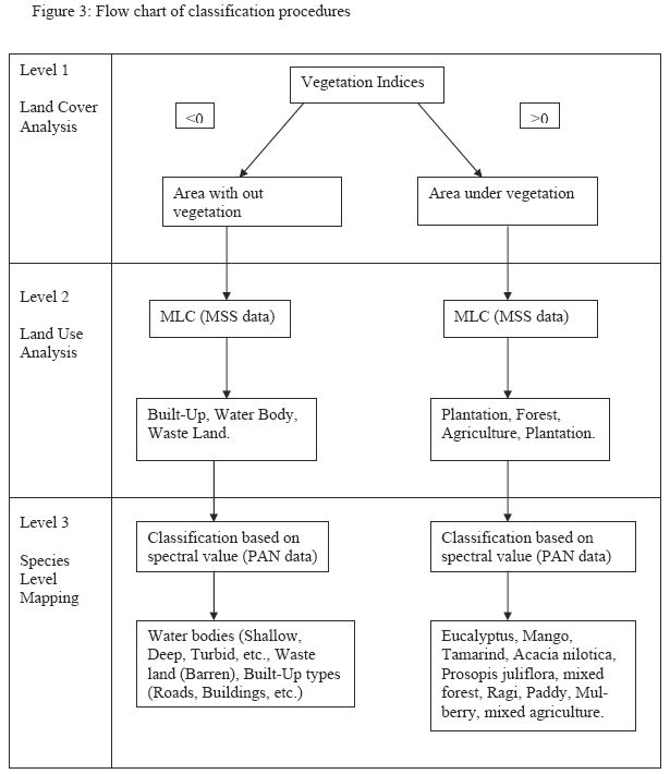
For land cover, land use and species level analyses hierarchical classification approach was adopted and the classification procedures are illustrated through a flow chart given in Figure 3.
Land cover analysis was done using different slope and distance based vegetative indices (VIs). This helps in identifying observed physical cover including vegetation (natural or planted). VI is computed based on the data grabbed by space borne sensors in the range 0.6-0.7 (red band) and 0.7-0.9 (Near-IR band), which helps in delineating the area under vegetation and non-vegetation areas.
It is found that vegetation is sparsely distributed in Kolar district because of its semi-arid environment and pixels contain a mixture of green vegetation and soil background. Hence, in addition to slope based vegetation indices, distance based vegetation indices have been computed. This would cancel the effect of soil brightness in case where there is mixture of green vegetation and soil background.
Slope based VIs computations are done using data acquired in visible red and near IR bands. These values indicate both the status and abundance of green vegetation cover and biomass. This is the first level of classification and aid in delineating areas under vegetation from non-vegetation.
RATIO vegetation indices (Rose et al.,1973) separate green vegetation from soil background by dividing the reflectance values contained in the near IR band (NIR) by those contained in the red band (R).
Ratio = NIR / RED ............................................ (1)This clearly shows the contrast between the red and infrared bands for vegetated pixels with high index values being produced by combinations of low red (because of absorption by chlorophyll) and high infrared (as a result of leaf structure) reflectance. Ratio value less than 1.0 is taken as non-vegetation while ratio value greater than 1.0 is considered as vegetation. The major draw back in this method is the division by zero. Pixel value of zero in red band will give the infinite ratio value. To avoid this situation Normalized Difference Vegetation Index (NDVI) is computed.
NDVI overcomes the problem of Ratio method (i.e. division by zero). It was introduced in order to produce a spectral VI that separates green vegetation from its background soil brightness using IRS 1C MSS digital data (Rose et al.,1974) and is given by,
NDVI = (NIR - RED)/(NIR + RED) ............................. (2)This is the most commonly used VI due to the ability to minimize topographic effects while producing a linear measurement scale ranging from 1 to +1.The negative value represents non vegetated area while positive value represents vegetated area.
The ratio vegetation index is the reverse of the standard simple ratio (Richerdson and Wiegand, 1977),
RVI= RED/NIR ...................(3)The range for RVI extends from 0 to infinity. The ratio value less than 1.0 is taken as vegetation while value greater then 1.0 is considered as non-vegetation area.
Normalized ratio vegetation index is a modification of the RVI (Baret and Guyot, 1991) where the result of RVI-1 is normalized over RVI+1.
NRVI=(RVI-1)/(RVI+1) ....................(4)
This normalization is similar in effect to that of NDVI, i.e it reduces topographic, illumination and atmospheric effects and it creates a statistically desirable normal distribution. Ratio value less than 0.0 indicates vegetation area while greater than 0.0 values represents non-vegetation.
TVI is modified version of NDVI to avoid operating with negative NDVI values (Deering et al., 1975). Adding 0.50 to NDVI value and taking the square root of the result computes TVI value. The calculation of the square root is intended to correct NDVI values approximate a Poisson distribution and introduce a normal distribution.

However negative values still exist for values less than 0.5 NDVI. There is no technical difference between NDVI and TVI in terms of image output or active vegetation detection. Ratio values less than 0.71 is taken as non-vegetation and value greater than 0.71 gives the vegetation area.
CTVI suppresses the negative values in NDVI and TVI (Perry and Lautenschlager, 1984). Adding a constant of 0.5 to all NDVI values does not always eliminate all negative values as NDVI values ranges from 1 to +1. Values that is lower than 0.50 will leave small negative values after the addition operation. Thus CTVI is intended to resolve this situation by dividing (NDVI+0.50) by its absolute value ABS (NDVI + 0.50) and multiplying the result by the square root of the absolute value (SQRT[ABS(NDVI + 0.50)]).

The correction is applied in a uniform manner, the out put image using CTVI should have no difference with the initial NDVI image or the TVI whenever TVI properly carries out the square root operation. The correction is intended to eliminate negative values and generate a VI image that is similar to, if not better than, the NDVI. Ratio value less than 0.71 is taken as non-vegetation and value grater than 0.71 gives the vegetation area.
The CTVI image is very noisy due to an overestimation of the greenness, which can be avoided by ignoring the first term of the CTVI, and it provides the better results (Thiam, 1997) .This is done by simply taking the square root of the absolute values of the NDVI in the original TVI expression to have a new VI called as TTVI. It can be defined as:
Ratio value less than 0.71 is taken as non-vegetation and value grater than 0.71 gives the vegetation area.

Distance Based VIs | TOP |
The main objective of the distance based vegetation index is to cancel the effect of soil brightness in cases where vegetation is sparse and pixels contain a mixture of green vegetation and soil back ground. This is particularly important in arid and semi-arid environment such as Kolar district of Karnataka.
Distance-based Vegetation indices are evaluated on the basis of soil line intercept concept. The soil line is a hypothetical line in spectral space that describes the variation in the spectrum of bare soil in the image. The soil line represents a description of the typical signatures of soils in red/near-infrared bi-spectral plot. It is obtained through liner regression of the infrared band against the red band for sample of bare soil pixels. Pixels falling near the soil line are assumed to be soils while those far away are assumed to be vegetation. Equation of the soil lines is given below,
Y1=0.841333x + 10.781234 (red band independent variable) ..................(8)
Y2=0.985684x + 9.501355(infra-red band as independent variable) ................(9)
The procedure requires that a set of bare soil pixels as a Boolean mask (value 1 is assigned to pixels representing soil while 0 for others). Analysis is done by regressing the red band against infrared band and vice versa. This provides slope and intercept of soil line. Distance based VIs using the soil line require the slope (b) and intercept (a) of the line as inputs to the calculation. Unfortunately there has been a remarkable inconsistency in the logic with which this soil line has been developed for specific VIs. For evaluating PVI2, PVI3, TSAVI1, TSAVI2, it requires red band as independent variable for the regression while for evaluating PVI, PVI1, DVI, WDVI and MSAVI requires infrared band as independent variable for regression.
PVI uses the perpendicular distance from each pixel co-ordinate to the soil line and this was derived to define vegetation and non-vegetation for arid and semi arid region (Richerdson and Wiegand, 1977). The pixels, which are close to soil line, are considered as non-vegetation while pixels, which are away from soil lines, represent vegetation. PVI values for data taken at different dates require an atmospheric correction of data, as PVI is quite sensitive to atmospheric variations. This can be defined as:
PVI= sin(a)NIR - cos(a)red ............................................. (10)
Where, a: Angle between the soil line and the NIR axis.

Where, (x1, y1) is the co-ordinate of the pixel and (x2, y2) is the coordinate of soil line point that is perpendicular to pixel co-ordinate.
Perpendicular distance less then 7.0 is taken as non-vegetation area while grater than 7.0 is taken as vegetation area.
It was noticed that original PVI equation is computationally intensive and does not discriminate between pixels that fall to the right or left of the soil line (i.e. water from vegetation). Given the spectral response pattern of vegetation in which the infrared reflectance is higher than the red reflectance, all vegetation pixels will fall to the right of the soil line. In some cases a pixel representing non-vegetation (e.g. water) may be equally far from the soil line but it will fall left side of the soil line.
In PVI the water pixel will be assigned a high vegetation index value. PVI1 assigns negative values to those pixels, which can be delineated from vegetation. The mathematical equation for PVI1 (Perry and lautenchlager, 1984) is written as,

Where, NIR: reflectance in the near infrared band, RED : reflectance in the red band, a : intercept of the soil line, b : slope of the soil line.
Infrared band is taken as the independent variable and the red band as dependent variable for regression analysis. Perpendicular distance less then 6.5 is taken as non-vegetation area while greater than 6.5 is taken as vegetation area.
In PVI2, Red band is taken as independent variable over infrared dependent variable for regression analysis (Bannari et al.,1996), given importance to the red band with the intercept of soil line. Mathematically PVI2 can be represented as,

Where, a: intercept of the soil line, b: slope of the soil line.
Here, pixels having less than 95.0 are grouped as non-vegetation area.
PVI3 is improved version of PVI, where red band is taken as independent variable on regression analysis and special attention was given to avoid the negative results (Qi et al.,1994). PVI3 can be defined as,
PVI3= apNIR bpRED ................... .(14)Where, a: intercept of the soil line, b: slope of the soil line, pNRI: reflectance in the near infrared band, pRED: reflectance in the visible red band.
DVI weigh up the near-infrared band by the slope of the soil line (Richerdson and Wiegand, 1997) and is given as :
DVI= gNIR RED .................... (15)Where, g: the slope of the soil line.
Similar to the PVI1, with the DVI, a value of zero indicates bare soil, values less than zero indicate non vegetation and greater than zero indicates vegetation.
AVI [19] is presented as a measure of growing green vegetation. Scaling factor is required for evaluating AVI. For IRS 1C data scaling factor of 1 was chosen, as all bands are 7-bit. AVI can be represented as,
AVI= sNIR RED .................... (16)Where, s: scaling factor.
AVI was evaluated for Kolar district using scaling factor as 1 for 8-bit MSS data set.
Soil reflectance spectra depend on type of soil. The vegetation indices computed earlier assume that there is a soil line, where there is a single slope in red-NIR space. However, it is often the case that there are soils with different red-NIR slopes in a single image. Also, if the assumption about the isovegetation line (parallel or intercepting at the origin) is not exactly right, changes in soil moisture (which move along isovegetation lines) will give incorrect answers for the vegetation index. The problem of soil noise is most acute when vegetation cover is low. The following groups of indices like SAVI, TSAVI1, TSAVI2, MSAVI1, MSAVI2 attempt to reduce soil noise by altering the behavior of the isovegetation lines. All of them are ratio-based, and the way that they attempt to reduce soil noise is by shifting the place where the isovegetation lines meet. These indices reduce soil noise at the cost of decreasing the dynamic range of the index. These indices are slightly less sensitive to changes in vegetation cover than NDVI (but more sensitive than PVI) at low levels of vegetation cover. These indices are also more sensitive to atmospheric variations than NDVI (but less so than PVI).
SAVI is intended to minimize the effects of soil background on the vegetation signal by incorporating a constant soil adjustment factor L in the denominator of the NDVI equation (Huete,1988). L varies with the reflectance characteristics of soil (i.e. color and brightness). The L factor chosen depends on the density of the vegetation. For very low vegetation L factor can be taken as 1.0 while for intermediate it can be taken as 0.5 and for high density 0.25. The best L value to select is where the difference between SAVI values for dark and light soil is minimal. For L=0, SAVI equals NDVI. For L=100, SAVI approximates PVI. Mathematically SAVI is defined as,
SAVI = {(NIR - RED) /( NIR+RED+ L)} * (1+L) .................... (17)
Where, NIR: near-infrared band, RED: visible red band, L: soil adjustment factor.
Multiplicative term (1+L) present in SAVI (and MSAVI) is responsible for vegetation indices to vary from 1 to +1. This is done so that both vegetation indices reduce to NDVI when the adjustment factor L goes to zero. Soil adjustment factor (L) of 0.5 was considered for Kolar district, as vegetation density is medium.
SAVI concept is exact only if the constants of the soil line are a = 1 and b = 0, where a is slope of the soil line and b is y-intercept of the soil line. As it is not generally the case some modification was needed in SAVI. By taking into the consideration of PVI concept (Baret et al., 1989), SAVI is modified as TSAVI1. This index assumes that the soil line has arbitrary slope and intercept, and it makes use of these values to adjust the vegetation index and is written as:

Where, NIR: reflectance in near infrared band, RED: reflectance in red band, a: slope of the soil line, b: intercept of the soil line, X: adjustment factor which is set to minimize soil noise.
Red band is taken as independent variable for regression analysis. Ratio value less than 9.0 is taken as non-vegetation while greater than 9.0 is taken as vegetation. With some resistance to high soil moisture, TSAVI1 could be very good candidate for use in semi-arid regions. TSAVI1 was specifically designed for semi-arid region and does not work well in areas with heavy vegetation.
TSAVI2 is modified version of TSAVI which was readjusted with an additive correction factor of 0.08 to minimize the effects of the background soil brightness (Baret et al., 1989), and is given by,

Red band is taken as independent variable for regression analysis and is given preference with soil line intercept.
The adjustment factor L for SAVI depends on the level of vegetation cover being observed which leads to the circular problem of needing to know the vegetation cover before calculating the vegetation index which is what gives you the vegetation cover. MSAVI is the Modified Soil Adjusted Vegetation Index (Qi et al.,), and provide a variable correction factor L. The correction factor used is based on the product of NDVI and WDVI. This means that the isovegetation lines do not converge to a single point. MSAVI1 is written as,

Where, L : 1 - 2 * s * NDVI * WDVI, s: slope of the soil line, NDVI: Normalized Difference Vegetation Index, WDVI : Weighted Difference Vegetation Index, 2 : Used to increase the L dynamic range, range of L = 0 to 1.
MSVI2 was derived based on a modification of the L factor of the SAVI (Qi et al.,). SAVI and MSVI2 are intended to correct the soil background brightness in different vegetation cover conditions. Basically, this is an iterative process and substitute 1-MSAVI (n-1) as the L factor in MSAVI (n) and then inductively solve the iteration where MSAVI (n)=MSAVI(n-1). MSVI2 uses an inductive L factor to :
The general expression of MSAVI2 is,

Where, NIR : reflectance of the near infrared band, RED: reflectance of the red band.
Pixel value less than 0.0 are under non-vegetation and pixel having greater than 0 are under vegetation.
Like PVI, WDVI is very sensitive to atmospheric variations (Richerdson and Wiegand, 1977) and can be presented as,

Where, NIR : reflectance of near infrared band, RED: reflectance of visible red band, g: slope of the soil line.
Although simple, WDVI is as efficient as most of the slope based VIs. The effect of weighting the red band with the slope of the soil line is the maximization of the vegetation signal in the near-infrared band and the minimization of the effect of soil brightness.
Land Use Analysis | TOP |
Land use analysis is done through classification of remotely sensed data. It requires the assignment of each of the pixels on an image to a class. The classification approach is based on the assumption that each of the classes on the ground has a class-specific spectral response and also each of the classes has varying spectral patterns. There is substantial variation in the distribution of the pixel reflectance values (depending upon samples location within a cover type). The spectral information contained in the original and transformed bands is then used to characterise each class pattern, and to discriminate between classes. There are two approaches to classify an image, namely Supervised and unsupervised classification techniques. Unsupervised classification technique intends to uncover the major land cover classes that exist in the image, without prior knowledge or field data. This is based on cluster analysis, considering clusters of pixels with similar reflectance characteristics in a multi-band image.
With supervised classification one provides a statistical description of the manner in which expected land use classes should appear in the imagery, and then the likelihood that each pixel belongs to one of these classes is investigated. Once a statistical characterisation has been achieved for each information class, the image is then classified by examining the reflectance for each pixel and making a decision about which of the signatures it resembles most. There are several techniques for making these decisions, and these are often termed classifiers (Hard and soft classifiers). Among Hard classifiers three approaches [Parallelepiped (PP), Minimum Distance to Mean (MD), and Maximum Likelihood (MLC)] were used to classify the images. The classified images were then reclassed into final six land use types. Different hard classification procedures are described below.
The Minimum Distance classification approach is commonly used when the number of pixels used to define the signatures is very small or when training sites are not well defined. By characterizing each class by its mean band reflectance only, it has no knowledge of the fact that some classes are inherently more variable than others, which in turn can lead to misclassification. Unknown pixels are classified based on its distance from the mean vector.
The parallelepiped procedure characterizes each class by the range of expected values on each band. This range may be defined by the minimum and maximum values found in the training site data for that class or by some standardized range of deviations from the mean with multi spectral image data, which ranges from an enclosed box-like polygon of expected values known as a parallelepiped. However, the performance of this classifier is very poor.
Maximum Likelihood Classification is one of the most widely used methods in classifying remotely sensed data. The MLC procedure is based on Bayesian probability theory. This technique generally yields higher accuracy in classification, but it is very computationally intensive and time consuming. It was found that maximum likelihood classification approach is the best of all the hard classifiers based on the accuracy assessment matrices (confusion matrices) generated for all the three classified images. Also MLC has generally been proven to be the one that obtains best results for classification of remotely sensed data. Hence, MLC approach was adopted for land use analysis. This provides classified information at both macro and micro level. For macro level classification training sites were selected so as uniformly distributed all over the taluk and about 375 training sites (GCP) were chosen for an area of 750-1000 sq. km. and remotely sensed MSS data were used. In case of micro level classification village wise training data at pixel level were collected and high resolution PAN data was used.
This classification is based on probability density function associated with a particular signature (training site). Pixels are assigned to most likely class based on a comparison of the posterior probability that it belongs to each of the signatures being considered. Mean and standard deviation for each training set is calculated. Probability density function is derived from mean and standard deviation and probability of each pixel belonging to each category is computed.
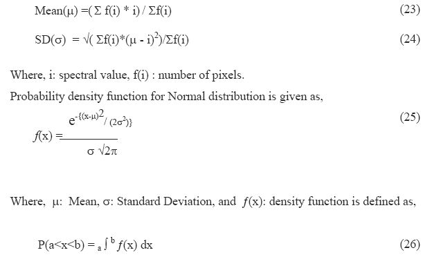
Where, a and b are minimum and maximum spectral values of training site respectively. The pixel is assigned to that training site, where its probability is found maximum. Further species level classification was done on the basis of spectral response pattern of different species, which is based on pixel level mapped field data.
The final stage of classification process usually involves an accuracy assessment. The purpose is to estimate the accuracy of quantification of mapping using remote sensing data to the ground conditions. This is useful in comparing classification techniques, and determining the level of error that might be contributed by the land cover image in further analyses in which it is incorporated. Accuracy of each classification is expressed as an error matrix. An error matrix is a square array of numbers in which the columns express the informational categories, and the rows show the classes in which those informational categories have been classified. The overall agreement of the classification is therefore expressed by the sum of main diagonal entries. An omission error happens when a test area that should have been classified into its informational category is not; on the other hand, the commission error occurs when a test area is classified in a class different from its true informational category. Information about these types of errors is given by the user's and producer's accuracies respectively. Test areas of the same size as the training areas were used to determine the agreement of the classification with the ground reference data. The majority rule was used to determine the class in which a test area is classified. With this rule, a test area is classified into the class that presents the highest frequency of pixels within the test area. The agreement of the classification with ground truth was measured by means of the overall accuracy, and the Kappa statistic.
Traditionally, accuracy assessment is done by generating a random set of locations to visit on the ground for verification of the true land cover type. A simple values file is then made to record the true land cover class (by its integer index number) for each of these locations. This values file is then used with the vector file of point locations to create a raster image of the true classes found at the locations examined. This raster image is then compared to the classified map using ERRMAT. ERRMAT tabulates the relationship between true land cover classes and the classes as mapped. It also tabulates errors of omission and errors of commission as well as the overall proportional error. This information is used to assess the accuracy of the classification procedure that was undertaken and is used for the results of all supervised classifications.
The size of the sample (n) to be used in accuracy assessment can be estimated using equation (3):

Where, z: the standard score required for the desired level of confidence, (i.e. 1.96 for 95% confidence, 2.58 for 99% etc) in the assessment, e: the desired confidence interval (e.g. 0.01 for 10%), p: the prior estimated proportional error and q = 1 p
Bioresource availability was computed considering the extent of land use in each category (like agriculture, forests, etc.) and the productivity. Overlaying a vector layer with taluk boundaries on the classified image of the district provides taulk level estimates. In order to assess the bioresource stock species wise, pixel level mapping was done using digitised cadastral maps of villages and GPS.
The area under different species was noted along with their location co-ordinates, vegetation types, etc. When two or more species coexisted, it was taken as mixed vegetation. Agriculture, plantation, forest and built up area were mapped at pixel level on the village maps. While, mapping areas under forest and plantation, parameters such as species type, canopy cover, girth at breast height (at 135cm height), height and density were also noted down (these parameters would be useful to assess the standing biomass). This field data (vector layer of villages ) is compared with the corresponding geo-referenced remote sensing data of spatial resolution 5.8 m (by overlaying these two layers). This helped in obtaining the spectral response pattern for species.
Bioresource mapping software was developed in C++ for finding the spectral range of each species and their corresponding spectral response pattern.
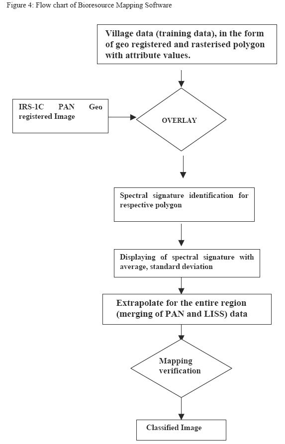
Bioresource Mapping Software | TOP |
Bioresource Mapping Software developed as illustrated in Figure 4 provides spectral response range of each species. This classification depends on probability density function associated with spectral signatures (spectral response pattern) of a particular species training site (micro level Maximum Likelihood classification). With the help of this software, the geo-registered vector layer of training data collected from sample villages (village level pixel mapping) was overlayed to its corresponding geo-registered PAN image. Training data in the form of polygons (each polygon representing a type of species) is overlayed to PAN image and the corresponding pixel values for the entire region is found out. The histogram is plotted for the dominant specie and probability density function was found out.
Histogram plays an important role in species level mapping. Vector layer of species (based on field data) was overlaid on raster image and corresponding spectral value was recorded and histogram generated for those species, which provides spectral range of the species. This can be narrowed down through statistical analyses (and considering parameters such as density or spatial spread of species, age of species, etc.). On the basis of the variability, new spectral range for the training site was selected. Based on these parameters, probability density function was determined which helps in classification.
Histogram analysis along with bioresource mapping software provides the spectral range for individual species. However, there is variation in spectral values due to seasonal aspects. It is found that spectral value of eucalyptus was 94-95 on 17th November 1998, while on 30th January 1999 the value changed to 86-88. Hence, season wise PAN scene classification has been done. Spectral range for each species was determined through probability density function. This information was used to classify the image and the result is extrapolated for the entire taluk and then to the district. This study maps the resources available in different levels- village, taluk and district.
Field survey in Kolar indicates that rural people depends on species such as Prosopis juliflora, Acacia nilotica, Acacia auriculiformis to meet fuel wood requirement for domestic activities. Detailed study was carried on for fuel wood species Prosopis juliflora - its spectral response pattern was found out with the help of bioresource software. Training data for Prosopis juliflora was taken from Iragasandra and Huttoor villages of Kolar taluk. Bioresource software provided its spectral range is 98-99. This spectral range was mapped in Kolar taluk and subsequently in Gauribidanur taluk (where training data was not collected) and cross verification was done in both taluks. Gauribidanur taluk, lies in north-western side of the district has basic soil and allows the growth of Prosopis juliflora, was chosen for mapping and verification of Prosopis juliflora.
Population data for the Kolar district is based on 2000 census data. For projections, it was assumed that average annual growth would remain the same as that recorded between 1980 and 1990, and 1990-2000. Village wise population data was collected and population density was calculated. It is found that population density is more and higher growth in towns compared to rural area.
The objective of the energy demand analysis is to develop a set of projections of future energy consumption. Two major approaches to energy demand analysis are macro and sectoral demand analysis. Macro demand analysis considers demand as a function of population, income, and prices. These data have been collected from secondary sources like different government agencies and different organisations. Sectoral demand analysis examines the structure of sectors and sub-sectors and their energy consuming activities. For evaluating, sectoral demand household survey was carried out. Total 2070 houses from all taluks of Kolar district were surveyed on the basis of questionnaire in different seasons like summer, winter, rainy and during different special occasions (like festivals). It is found that demand (per capita fuel consumption) in this region varies from 1.3 kg/person/day to 2.5 kg/person/day. Based on the primary and secondary data, bioresource status was calculated for each village.
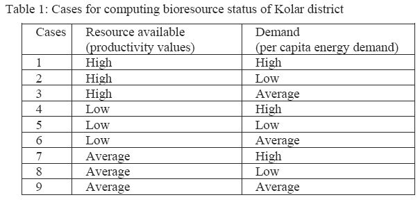
The ratio of availability to the demand (bioresources) gives an idea of its status in a region. The resource availability to the entire district is done in cost and time effective way with the help of spatial and temporal tools such as GIS, Remote sensing data and collateral data. Hierarchical classification techniques used in analysing remote sensing data provided details about land use and the area under each vegetation (at species level). Based on the productivity value ranges for forest/plantation, bioresource availability is computed as Resource (average), Resource (high) and Resource (low) categories. Bioresource productivity in each type of landuse is computed based on field sampling techniques. Based on randomly selected quadrant in all types of land use, the productivity ranged from 3.6 to 6.5 tonne/hectare/year for evergreen, 13.5 to 27 ton/hectare/year in deciduous patches and 0.8 to 1.5 tonne/hectare/year for scrub jungle.
Bioresource demand estimation is based on randomly selected sample households (2070 houses using standard questionnaire). These houses were selected from 154 villages, which are situated all over Kolar district covering different community and category of people (stratified random sampling). Seasonal survey was carried out to find out the season wise variation apart from the estimation of fuelwood demand during different festivals. On the basis of the field data collected from different seasons average energy consumption per person was estimated, which gives an average demand value.
Based on the three cases for resource availability and three cases for demand, the bioresource status (ratio of bioresource availability to demand) for the Kolar district was computed for nine different combinations as listed in Table 1. The value of bioresource status greater than one indicates that the region has surplus resources, while values less then one indicate bioresource scarcity.
 | TOP |