|
Results and Discussion
Temporal NDVI analysis shows reduction of region under vegetation by 7.27% from 1972 to 2000 and a decrease of 4.72% from 1972 to 2007. Histograms were generated to ascertain the number of likely LU categories based on the number of distinguishable peaks. Six distinct classes: agriculture, settlement, forest, plantation/orchard, barren land and water were the dominant categories in the study area. Signatures were assessed using spectral graphs which showed that forest and plantation/orchard classes have high peaks in the NIR band and are therefore distinguishable from other classes. In band 3 of Landsat MSS settlement and dry river bed were not distinguishable, whereas in Landsat ETM+ for the same band, river bed was not easily distinguishable from barren land/stony/waste. In LISS III, settlement and barren land signatures were not separable in band 3. All other classes were well separable. Supervised classification (figure 2) with the percentage statistics are listed in table 1.
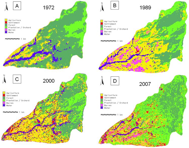
Figure 2: Classification using (A) Landsat MSS, 1972, (B) Landsat TM, 1989, (C) Landsat ETM, 2000 and (D) IRS LISS-III, 2007.
Table 1: Spatio-temporal LU estimates
| |
Class →
Area ↓ |
Agriculture |
Built-up |
Forest |
Plantation / Orchard |
Barren land |
Water |
Total |
| 1972 |
Area (Ha) |
215.88 |
- |
855.21 |
204.25 |
15.02 |
115.42 |
1405.8 |
| Area (%) |
15.36 |
- |
60.84 |
14.53 |
1.07 |
8.21 |
100 |
| 1989 |
Area (Ha) |
559.39 |
3.26 |
395.28 |
267.39 |
117.17 |
63.29 |
1405.8 |
| Area (%) |
39.79 |
0.23 |
28.12 |
19.02 |
8.33 |
4.50 |
100 |
| 2000 |
Area (Ha) |
495.80 |
104.41 |
467.76 |
209.54 |
13.66 |
114.62 |
1405.8 |
| Area (%) |
35.27 |
7.43 |
33.27 |
14.91 |
0.97 |
8.15 |
100 |
| 2007 |
Area (Ha) |
249.81 |
98.74 |
318.17 |
640.45 |
55.15 |
43.45 |
1405.8 |
| Area (%) |
17.77 |
7.02 |
22.63 |
45.66 |
3.92 |
3.09 |
100 |
Accuracy assessment is listed in table 2. ROC curves for each class for the temporal dataset in figure 3 show the performance of the classifier as the decision threshold is varied for each class to obtain the best classified output. At any point on the curve is a possible operational point for the classifier and so was evaluated in the same manner as accuracy. There is a good agreement between results obtained from error matrix and ROC curves.
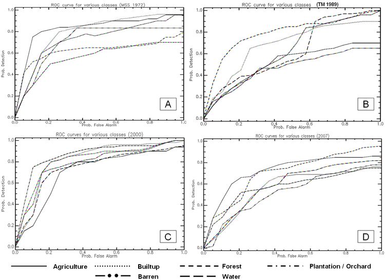
Figure 3: ROC curves for [A] Landsat MSS-1972; [B] Landsat TM – 1989; [C] Landsat ETM+ - 2000; [D] LISS-III - 2007.
Table 2: Accuracy assessment for classified images
| Class |
1972 |
1989 |
2000 |
2007 |
| Accuracy→ |
PA* |
UA* |
PA |
UA |
PA |
UA |
PA |
UA |
| Agriculture |
70 |
75 |
80 |
83 |
87 |
84 |
90 |
85 |
| Builtup |
60 |
65 |
76 |
71 |
83 |
82 |
86 |
81 |
| Forest |
86 |
81 |
85 |
80 |
91 |
87 |
90 |
85 |
| Plantation/ Orchard |
73 |
78 |
85 |
77 |
87 |
85 |
91 |
87 |
| Barren |
80 |
82 |
84 |
84 |
80 |
79 |
88 |
86 |
| Water |
83 |
82 |
78 |
75 |
83 |
82 |
83 |
78 |
| OA* |
78.52 |
80.78 |
83.78 |
86.52 |
| Kappa |
0.7735 |
0.8066 |
0.8217 |
0.8667 |
*PA - Producer’s Accuracy, UA - User’s Accuracy, OA - Overall Accuracy
Results obtained from MLC classification are comparable to the ground condition for the 2007 classified image. The successful application of MLC is dependent upon having delineated correctly the spectral classes in the image data of interest. This is necessary since each class is to be modeled by a normal probability distribution. If a class happens to be multimodal, and this is not resolved, then clearly the modelling cannot be very effective. MLC can obtain minimum classification error under the assumption that the spectral data of each class is normally distributed. The disadvantage of this technique is that it requires every training set to have at least one more pixel than the number of bands used in classification.
Forest patches have declined from 61 ha (in 1972) to 23 ha (in 2007) with the conversions of forest for agricultural activities, which has significantly increased by ~20% from 1972 to 2000. However, the percentage area pertaining to agriculture has decreased to 17% in 2007. One of the reasons is that agricultural area and fallow land were invaded by an exotic weed – Lantana camera which is an invasive species that thrives in warm, high rainfall areas where it forms dense thickets that exclude native species through shading and allelopathic effects, leading to complete dominance of the under storey and eventually overshooting the main canopy. The thickets impede access, alter availability of fodder for wild animals and reduce regeneration potential displacing natural scrub communities. Lantana encroaches agricultural land, reduces the carrying capacity of pastures. Its distribution has adversely affected not only many species of economic and ecological importance but ecosystem also. Plantation has increased considerably from ~15% (1972) to ~46% (2007). These include Babool, Acacia catechu and shrubs as a government measure to retain greenery in the area. Barren lands mainly constitute rocks, stones and open lands. Some of the barren land pixels show similar reflectance as that of dry river bed and the signatures often mix with settlements causing confusion during classification. Hence the proportion of barren land is less compared to earlier classified images (from 1989 to 2007).
Change detection involved differencing images of two time periods between PCs, CA components, NDVI and bands (rescaled from -1 to 1) that showed similar results. In both the images of the standardised PCA, PC1 had the highest information having all bands with unequal variances. CA puts less emphasis on bands that have low polarisation. The more the pixels are polarised for a band, the higher the importance given to that band in the calculation of the between-pixel distances (Greenacre, 1984). The first two components of CA explained approximately 99% of the total inertia in both temporal images (table 3). Total inertia is a measure of how much the individual pixel values are spread around the centroid. Inertia is independent of the absolute frequencies that constitute the original data, and will be identical if the data are multiplied by any constant value (Greenacre, 1984).
Table 3: Eigen structure of 1972 and 2007 data after PCA and CA transformation
PCA |
|
Landsat MSS (1972) |
IRS LISS-III (2007) |
| |
Comp1 |
Comp2 |
Comp3 |
Comp1 |
Comp2 |
Comp3 |
| Band 1 |
0.66 |
0.24 |
0.71 |
0.62 |
0.33 |
0.71 |
| Band 2 |
0.66 |
0.28 |
-0.70 |
0.62 |
0.36 |
-0.70 |
| Band 3 |
0.37 |
-0.93 |
-0.02 |
0.49 |
-0.87 |
-0.01 |
| Eigenvalues |
2.14 |
0.82 |
0.03 |
2.44 |
0.55 |
0.01 |
| Proportion |
72 |
27 |
1 |
81.25 |
18.26 |
0.48 |
| Cumulative |
72 |
98 |
100 |
81.25 |
99.51 |
100 |
Correspondence Analysis |
|
Landsat MSS (1972) |
IRS LISS-III (2007) |
| |
Comp1 |
Comp2 |
Comp3 |
Comp1 |
Comp2 |
Comp 3 |
| Band 1 |
0.62 |
0.24 |
0.75 |
0.58 |
0.27 |
0.77 |
| Band 2 |
0.60 |
0.47 |
-0.65 |
0.58 |
0.53 |
-0.62 |
| Band 3 |
0.51 |
0.85 |
-0.15 |
0.57 |
-0.81 |
-0.15 |
| Eigenvalues |
2.50 |
0.50 |
0.006 |
2.96 |
0.037 |
0.0002 |
| Proportion |
83.23 |
16.57 |
0.2 |
98.76 |
1.23 |
0.0066 |
| Cumulative |
83.23 |
99.80 |
100 |
98.76 |
99.99 |
100 |
Detailed change detection tabulation was done between two classified images of 1972 and 2007 focusing primarily on the initial state classification changes – that is, for each initial state class, it identifies the classes into which those pixels changed in the final state image. The total class change for agriculture is 135.81 ha. There is a decrease of 537.03 ha in forest class and there has been an increase of 436.22 ha in plantation / orchard class. Forest fragmentation maps along with associated statistics based on the temporal forest maps (LU analysis) are presented in figure 4 and table 4.
Table 4: Forest fragmentation types details
| |
1972 |
1989 |
2000 |
2007 |
| |
Ha |
% |
Ha |
% |
Ha |
% |
Ha |
% |
| Interior |
751.89 |
90.36 |
337.83 |
86.45 |
336.83 |
75.24 |
106.06 |
33.35 |
| Perforated |
48.00 |
5.77 |
38.96 |
9.97 |
73.85 |
16.50 |
20.98 |
6.60 |
| Edge |
25.58 |
3.07 |
9.53 |
2.44 |
24.02 |
5.37 |
122.07 |
38.39 |
| Transitional |
6.66 |
0.80 |
4.45 |
1.14 |
12.97 |
2.90 |
46.01 |
14.47 |
| Patch |
- |
- |
- |
- |
0.01 |
0.00 |
22.85 |
7.19 |
| Total |
832.15 |
100 |
390.78 |
100 |
447.68 |
100 |
318.01 |
100 |
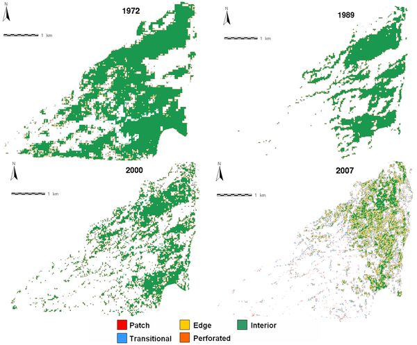
Figure 4: Forest fragmentation maps for 1972, 1989, 2000 and 2007.
Total forest proportion (TFP) and forest continuity (FC) is listed in table 5 and are depicted in figure 5. The forest fragmentation metrics analysis showed that largest forest patch is continuously decreasing consequently increasing the number of small patches and patch density. Due to increasing number of patches, more edges are getting developed with increasing edge density and the landscape shape is becoming more complex with time.
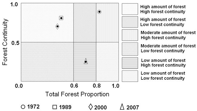
Figure 5: Six forest fragmentation conditions based on the values for TFP and FC.
Table 5: Total forest area and weighted forest area
| |
1972 |
1989 |
2000 |
2007 |
| TFP |
0.82 |
0.49 |
0.53 |
0.70 |
| FC |
0.88 |
0.84 |
0.71 |
0.26 |
The results of this study based on the temporal remote sensing data supplemented with the field data indicate that Mandhala watershed is degrading due to intense anthropogenic activities. When anthropogenic causes of fragmentation are considered, forest are more likely to be disturbed and fragmented where climate is hospitable, soil is productive and access is easy. Mandhala watershed is under the severe influence of forest fragmentation, calling for immediate protection measures from the concerned authorities.
|
