5 . 1 . 1 Agent-based Modelling Using the Tool - NetLogo
| Back |
5 . 1 Implementations of Agent-based Models for Simulating Urban Sprawl
Simulating a dynamic phenomenon like the urban sprawl using the agents in conjunction with the CA models was attempted in this research. The framework for ensuring the simulations developed in the Chapter 3 and the dynamics of urban sprawl studied and modelled using CA and agents in the Chapter 4 are implemented. Accordingly, there are two agent-based modelling approaches for simulating urban sprawl. In the first approach, much before researchers started to use the agent-based models in the geo-spatial domain, architecture and tools for building the agent-based models were developed (Chapter 2). Hence, much of the development and applications was restricted to the software engineering domain, until user-friendly tools for building agent-based models emerged in research and industry. However, with the application of agent-based modelling for geo-spatial processes, few researchers have attempted to fuse the agent-based models over a GIS (Batty, 2003; Benenson and Torrens, 2003). Using the first approach, NetLogo (Wilensky, 1999) (tool for building agent-based models) was used to demonstrate the capabilities of agent-based modelling techniques for studying urban sprawl dynamics. In this approach no actual geo-spatial data was used. Just a prototypical situation of a city exhibiting urban sprawl in radial direction was demonstrated. In the second approach, agent-based models operated on geo-spatial data and were applied for a region experiencing a high rate of urban sprawl. The ensuing sections discuss on the implementations of the same.
5 . 1 . 1 Agent-based Modelling Using the Tool - NetLogo |
The agent-based modelling tool NetLogo developed by the Centre for Connected Learning and Computer Based Modelling, Northwestern University, USA was used to demonstrate a prototypical simulation of the urban sprawl in radial direction. In the NetLogo parlance the agents are conceived as turtles', the sense of state is through patches' and the worldview through the observer' (Wilensky, 1999). Patches are similar to the notion of cell in CA with the regular lattice structure. Each cell in the CA terminology corresponds to the patch in the NetLogo parlance. Thus, the notion of space is based on regular lattice structures of square cells and agents are simulated to move over a cellular space.
A prototype city was created by patches in the centre of a worldview of 29 x 29 cells. Several types of agent-hood (Jennings and Wooldridge, 1996), autonomy, social ability, responsiveness and pro-activeness are attributed to the turtles to operate in these patches. The developed called built-up' is attributed as one type of agent or turtle in this case. The other agents include available land for development as land'. The built-up agent is represented by the graphic shown in red colour as a house, while the land agent is represented by the graphic shown in brown colour as a box over the patches. In order to establish a hypothetical city exhibiting radial urban sprawl, the model is initialised having a city with built-up as core area at the centre and the land with the scope for development spread surrounding the core region. For setting up the model or creating this instance of having a city in the centre and the available land around it, the agents in this context, built-up and land were defined appropriately. The built-up agents are programmed to populate in the centre of the monitor depending upon the size of the city. A monitor is the space where all the patches are visualized, which in this case is 29x29 matrices of cells. The size of the city is controlled by its radius', which is scaled from 1 to 5 cells from the core region. For testing the rate of development that may take up depending upon the various sizes of the city and the nature of growth, the amount of land to built-up percentage can also be initialised by the user. An option to set the rate of development as built-up growth' in terms of percentage growth for each simulation time can also be initialised. There are adequate monitors in the prototype model to indicate the advancement of simulation time, number of land agents and number of built-up agents. An initialised model for simulation is as shown in Figure 5.1.

Figure 5.1: Initialised Model for Simulating Radial Urban Sprawl
In this model, the built-up agents are programmed so that they would populate or breed' in the agent-parlance if there exists a patch in its immediate neighbourhood with the land' agent occupied in it. The user can also set the radius of the neighbourhood from 1 to 5 cells using a 3x3 to 7x7 kernel. Within this predefined neighbourhood these built-up agents would be prioritised depending on whether the patch is already occupied by an agent. If a built-up agent has already occupied the patch, the agent would look for another patch. Thus the simulation of this model would go on until all the land is consumed in the neighbourhood.
The simulation output of the model demonstrating the radial urban sprawl is shown in Figure 5.2. From the model execution, various parameters like the nature of sprawl taking place and the rate of consumption of land over time are computed. From the model interface, it is evident that the agent actions can be continuously obtained in terms of their numbers over time. Further, for testing different scenarios and the implications of such scenarios can be easily visualised and quantified for various space-time variant phenomena like the urban sprawl. Traditional GIS currently doesn't support the understanding of space-time variant phenomena, the way agent-based models do. It was evident from the prototypical demonstration of the radial sprawl, that it was possible to visualize and quantify the variable state changes over space and time, which the traditional GIS being static does not allow to handle such data nor visualise them. However, with a possible convergence of the agent-technology with the GIS, analysing the patterns of change through time (Peuquet, 1999) can be a reality. Thus the agent-based models in the geo-spatial domain can be of more utility than also being just used for geo-spatial simulations.

Figure 5.2: Simulation of the Model for Demonstrating Radial Urban Sprawl
The time advancement mechanism in this case is by asynchronous updating. In such scenario, the cell updates would depend on the order of the agent execution that would take place as defined in the program flow.
The hypothetical model discussed earlier, serves to visualise the growth. This model can also be of use for teaching and demonstration purposes, while for an effective utilisation of the agent-based models in the geo-spatial domain the ensuing section addresses the implementation of the same.
5 . 1 . 2 Agent - based Modelling Using the Agent-Builder Interface |
With a prototype demonstration of a hypothetical situation of radial urban sprawl, the research aimed at demonstrating a prototype for the simulation of urban sprawl for a real case in the geo-spatial domain. For the demonstration of the prototype simulations, the run-time infrastructure based on the HLA was not utilized in the simulation since the impending time constraint for implementation. However, the simulations in this research were undertaken in the geo-spatial environment, using a combination of GIS tools and spreadsheets for undertaking simulations were loosely coupled. The database on the demography remained in the Microsoft ® Excel format as a spreadsheet, while the remote sensing images were in IDRISI 32's *.rst format. IDRISI 32 provides an application program interface (API) for customization using Visual Basic (Eastman, 1999). This helped in first implementing the CA model loosely coupled with the IDRISI 32 raster GIS. In the next stage the agents were introduced. The implementation of the agent-action for such simulation first involved the development of an agent-builder interface. The utility and the scheme for building agents in geo-spatial domain has been discussed earlier (Chapter 4). On these lines for building agents, the interface was developed using the MapObjects2 developed by Environmental Systems Research Institute (ESRI) and Visual Basic, as illustrated in Figure 5.3. With the creation of agents in geo-spatial environment, this was coupled with the simulation model developed for CA in IDRISI 32. During the simulation execution, the simulation executive ensures the agents to interact with the CA model and initiate the transitions.

Figure 5.3: Prototype of the Agent Builder Interface
5 . 1 . 3 Rules for Agent Behaviour |
As mentioned in Chapter 4, the agents considered in this research model the population development process and the infrastructure. Knowing the behaviour of these agents, the same were programmed and executed according to the specific duration of these agent actions. The agent behaviour involved initiating state transitions in conjunction with the CA transition rules and responding certain criteria set by the modeller.
The specific rules that were formalized for the agents were based on the characteristics of sprawl observed in relation to the population and built-up density of the study area. It can be seen that when the population change was only about 50 %, the corresponding built-up change was about 150 %. This behaviour itself was formalized for the new built-up agents and the population development process. And so, for every change in population by 1 percent the built-up would change by 3 percent and vice versa. That is, for every increase in population of the region to increase by 1 percent, corresponding increase in built-up is by 3 percent. This in itself forms the feedback of interactions among the agents.
A scheme of the interaction of these agents and their initiation and responses to the transition rules of the CA are shown in Figure 5.4. A prototype scenario of such activities manifested by the agents and their interactions with the CA is initialized. In the prototype scenario, the creation of ring road by the user is seen as a first step. With this activity becoming into reality over a period of 4 years, other activities like the residential and industrial layouts follows. Simultaneously the population development process also picks up the rule governing the agent behaviour described earlier. Accordingly, the impacts of agent interactions are evident from the final simulations.
Figure 5.4: Interactions of the Agents with the CA Transition Rules
The features created as a shapefile using the interface, defines the extent of influence of the agents. Figure 5.5 shows the example creation of an agent extent using the interface, which is subsequently saved as a shapefile. In the next step, the attribute information of the duration of activity for these features is added. With this, these features were initialized for the image of the entire region as a binary image in the raster format compatible with IDIRSI 32, which were used in the simulations subsequently.
The flow of the simulation involves that with this addition of infrastructure, other allied activities like the industrial and residential layouts emerge with a resulting population growth. The agents' actions in conjunction with the CA transitions continuously manifest in order to achieve the equilibrium for the agent behaviour described. The visualization of such scenarios is presented in the subsequent section.
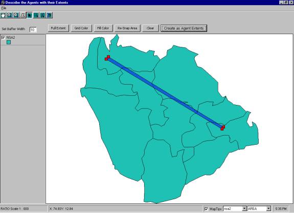
Figure 5.5: Example of Creation of Agent Extents using the Agent Builder Interface
5 . 2 Calibration and Validation |
Calibration is the iterative process of comparing a model to the real system, making changes to the parameters of the model, comparing the revised model with the reality, and making necessary changes, if required. Validation is the overall process of comparing the model and its behaviour to the real system and its behaviour (Banks and Carson, 1984). Essentially calibration helps in fixing the parameters of the model considered to appropriately represent the real system under investigation. In the current research, the calibration of the model by using the agents with the CA model was undertaken. In order to achieve this, the parameters considered for the CA model were to be adjusted to reflect the real system. In the foregoing sections the calibration and subsequent results of the simulations are discussed.
5 . 2 . 1 Calibration of the CA model |
The calibration of the CA model had to be done for the parameters considered to ensure that the model is reflecting the actual phenomenon under investigation. In the current set up, the abstraction of the CA model is as shown in Figure 4.4 . For the CA model to reflect the reality appropriately, the calibration was undertaken for the establishing the suitability appropriately by adjusting the factor weights. The multi-criteria evaluation in the IDRISI 32 was utilised for the adjusting the factor weights appropriately.
Initially the simulation was undertaken for a set of default values in the entire model. The simulation was undertaken from the year 1987 to 1999 that was for 12 iterations. With the available remote sensing imagery, IRS LISS-III for 1999, the simulation output of the CA model was evaluated for the accuracy of the simulations. By iteratively, adjusting the factors and factor weights, the calibration was done. Figures 5.6 and 5.7 shows the actual built-up for 1999 and simulated built-up, after reasonable calibration. Accuracy of the simulated built-up with respect to actual built-up was done by randomly selecting four 7x7 kernel window size within the region, to check whether the pixels were correctly assigned or not in the corresponding images. Of the 196 pixels, 134 of them were found to be properly assigned with respect to the reference image of 1999, indicating an accuracy of about 68.4 %. It can be seen that the calibration could only achieve a reasonable accuracy in the sprawl simulation while a higher efficiency of calibration could be performed with more parameters and more effort.
5 . 3 Simulation Results and Discussion |
With the calibration of the CA model, the simulation was undertaken until 2011, which corresponds to12 iterations for a scenario of an infrastructure like a ring road. The results are as shown in Figures 5.8 to 5.19. The simulations were undertaken using the calibrated CA transition rules and the transitions initiated by the ring road agent in this case.
It is noticed that the creation of infrastructure had its effect in the year 2003 (Figure 5.11), while the agent automata had initiated the cell transitions in the region of the ring road. Subsequently, for the transition the cell update takes in to account of any updates by the agent transitions. Figure 5.15 corresponding to year 2007 indicate that the region around the ring road showed considerable growth. By 2011 as indicated in the Figure 5.19, the region around the ring road is seen with significant development. It was observed that transition of non-built-up to built-up cell states has also occurred in the whole of the region, while a stronger growth was observed in the region around the ring road.
|
|
|
|
|
|
|
|
|
|
|
|
With the above simulations combining the CA and agent automata for the cell transitions, the visualization of the future scenario of urban growth by the creation of an infrastructure was successful. However, for an effective utilization of the agent hood in the simulation, adequate agents could be devised to report the nature of changes during the iterations. In this work, one aspect of the agent hood was demonstrated while for an effective realization of the agent properties in the geo-spatial simulations, further research is required.