4.1.1 Forms of Sprawl
| Back |
Economic activities coupled with new infrastructure to meet the requirements of unprecedented population growth and migration into urban centres has resulted in urbanization. More and more towns and peri-urbans are blooming with a change in the land use along the highways and in the immediate vicinity of the city due to adhoc approaches in decision-making. This dispersed development outside of compact urban and village centres along highways and in rural countryside is defined as sprawl and is devoid of basic amenities consequent to the adhoc approaches in planning. Hence, dynamics of sprawl needs to be understood in terms of the rate and pattern of growth to plan basic amenities.
Urbanization is a form of metropolitan growth that is a response to often bewildering sets of economic, social, and political forces and to the physical geography of an area. Some of the causes of the sprawl include - population growth, economy, patterns of infrastructure initiatives like the construction of roads and the provision of infrastructure using public money encouraging development. The direct implication of such urban sprawl is the change in land use and land cover of the region.
Sprawl generally infers to the increase in built-up and paved area with impacts such as loss of agricultural land, open space, and ecologically sensitive habitats. Also, sometimes sprawl is equated with growth of town or city (radial spread). In simpler words, as population increases in an area or a city, the boundary of the city expands to accommodate the growth; this expansion is considered as sprawl. Sprawl also takes place on the urban fringe or the peri-urban region, at the edge of an urban area or along the highways.
The sprawl results in the growth of villages into peri-urban areas, peri-urban areas to towns, towns into cities and cities into metros. However, in such a phenomenon of development to have basic infrastructure, regional planning requires an understanding of the sprawl dynamics. However, in majority of the cases there are inadequacies to ascertain the nature of uncontrolled growth. Sprawl is considered to be an unplanned outgrowth of urban centres along the periphery of the cities, along highways, along the road connecting a city, etc. Due to lack of prior planning these outgrowths are devoid of basic amenities like water, electricity, sanitation, etc. resulting in inefficient and drastic change in land use affecting the ecosystem (Sudhira et al., 2004a).
4.1.1 Forms of Sprawl |
Sprawl development consists of three basic spatial forms: low-density (radial) sprawl, ribbon and leapfrog development (Barnes et al., 2001). Radial sprawl is the consumptive use of land for urban purposes along the margins of existing metropolitan areas. This type of sprawl is supported by piecemeal extensions of basic urban infrastructures such as water, sewer, power, and roads. Ribbon sprawl is development that follows major transportation corridors outward from urban cores. In this case, lands adjacent to corridors are developed, but those without direct access remain in rural uses/covers. Over time these nearby raw lands maybe be converted to urban uses as land values increase and infrastructure is extended perpendicularly from the major roads and lines. The leapfrog development is a discontinuous pattern of urbanisation, with patches of developed lands that are widely separated from each other and from the boundaries, albeit blurred in cases, of recognised urbanised areas (Barnes et al., 2001). This form of development is the most costly with respect to providing urban services such as water and sewerage. Figure 4.1 shows the different forms of sprawl.
In industrialized countries the future growth of urban populations will be comparatively modest since their population growth rates are low and over 80% of their population already live in urban areas. Conversely, developing countries are in the middle of the transition process, when growth rates are highest. The exceptional growth of many urban agglomerations in many developing countries is the result of a threefold structural change process: the transition away from agricultural employment, high overall population growth, and increasing urbanization rates (Grubler, 1994).
Geo-informatics is very useful in the formulation and implementation of the spatial and temporal development strategies, which are essential components of regional planning to ensure the sustainable development. The different stages in the formulation and implementation of a regional development strategy can be generalized as determination of objectives, resource inventory, analysis of the existing situation, modelling and projection, development of planning options, selection of planning options, plan implementation, and plan evaluation, monitoring and feedback ( Yeh and Xia, 1996 ). The geo-spatial techniques are evolving for implementation of such a proposed strategy. The spatial patterns of urban sprawl on temporal scale is analysed and monitored using the remotely sensed satellite imageries. The image processing techniques are also quite effective in identifying the urban growth pattern from the spatial and temporal data. These help in delineating the growth patterns of urban sprawl such as, the linear growth and radial growth patterns.
Prior visualizing of the trends and patterns of growth enable the planning machineries to plan for appropriate basic infrastructure facilities (water, electricity, sanitation, etc.). The study of this kind reveals the type, extent and nature of sprawl taking place in a region and the drivers responsible for the growth. This would help developers and town planners to project growth patterns and facilitate various infrastructure facilities.
Mapping and quantification of urban sprawl provides a "picture" of location of sprawl, type and patterns of sprawl, which helps to identify the environmental and natural resources threatened by such sprawls. Analysing the sprawl over a period of time will help in understanding the nature and growth of this phenomenon and thereby visualizing the likely scenarios of future sprawl (Sudhira et al., 2004a).
In the recent years, a lot of thrust in this field has been to understand and analyse the urban sprawl pattern. Various analysts have made considerable progress in quantifying the urban sprawl pattern (Theobald, 2001; Torrens and Alberti, 2000; Batty et al., 1999). However, all these studies have come up with different methodologies in quantifying sprawl. The common approach is to consider the behaviour of built-up area and population density over the spatial and temporal changes taking place and in most cases the pattern of such sprawls is identified by visual interpretation methods.
Defining this dynamic phenomenon with relative precision and accuracy for predicting the future sprawl is indeed a great challenge to all working in this arena. The study of urban sprawl ( Sierra Club, 1998 ) is attempted in the developed countries (Batty et al., 1999; Torrens and Alberti, 2000; Barnes et al., 2001, Hurd et al., 2001; Epstein et al., 2002) and in developing countries such as China (Yeh and Li, 2001; Cheng and Masser, 2003) and India (Jothimani, 1997; Lata et al., 2001; Subudhi and Maithani, 2001; Sudhira et al., 2003). However there are very few studies on modelling urban sprawl are attempted (Subudhi and Maithani, 2001; Sudhira et al., 2004b). Although the notion of developed and developing countries is not crucial, the impacts of urban sprawl are ultimately on the regions land use mainly resulting in loss of prime agricultural lands and water bodies.
Although it is often considered endemic the phenomenon has impacts on the structure and growth of any city or town. Development of suburbs as a consequence of increased population growth and infrastructure facilities around the cities is a well-established reasoning for urban sprawl. Batty et al. (1999) have demonstrated the urban sprawl phenomenon as a spatially aggregate model. Various analysts have worked on urban growth modelling considering the spatial and temporal analyses of land use / land cover changes (LUCAS, GIGALOPOLIS, RESACC). However few analysts have made significant contributions on the urban sprawl dynamics (Batty et al., 1999; Torrens and Alberti, 2000).
The phenomenon of urban sprawl is very dynamic in nature. A complex of activities involving the economics, infrastructure addition, population growth and so on mainly attributes the urban sprawl dynamics. In this case, the different drivers are modelled as agents. The different drivers or the agents for inducing sprawl can manifest the sprawl by the complex of interactions and responses amongst them. The interactions among the agents of sprawl like the population or infrastructure can be complimentary to each other. Subsequently the reactions of these agent manifestations can lead to fuel further sprawl. Further, these agent-behaviours are not same with space and time; in effect these agents have an impact over system dynamically both in space and time. Visualizing such multi-scale space-time dynamic phenomenon like the urban sprawl is still not well handled by the traditional GIS (Batty, 2003).
Till date CA has been applied for simulating urban growth considering some of the driving forces responsible for sprawl. However some of the issues like the impact on socio-economic factors and policy matters are to be evaluated effectively while addressing issues like urban sprawl. For an effective simulation of the urban sprawl, modelling has to be attempted in both spatial and non-spatial domain. Most of the work in modelling the urban sprawl in the non-spatial domain is by the application of statistical techniques while CA models are known for modelling in spatial domain. In the recent years, the agent-based models in conjunction with the CA are used to represent the dynamics responsible for simulating scenarios of future urban sprawl (Chapter 2).
In this study the urban sprawl for a region is studied and modelled for the dynamics driving the sprawl using CA with agent-based models in the geo-spatial domain. The framework for integration of agent-based models over a CA model is discussed in the previous chapter. Before taking up the discussions on building the agent-based models, the abstraction of CA model is discussed. The agents are then integrated over the CA model.
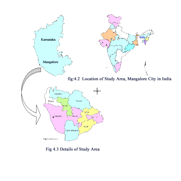
4.1.2 Description of Study Area- The Mangalore City |
This study was carried out in Mangalore, Karnataka, India (Figure 4.2). Mangalore, being a coastal city facing the Arabian Sea and the presence of a natural harbour, this has been one of the major ports of western coast of India. This region gains importance for the numerous financial institutions and hence has brisk economic activity as evinced from the growth of cities and infrastructure developments. In the recent years (post 1999), a lot of economic activity has been evinced with the boom in the information technology (IT) in the region. With the capital of the state, Bangalore, getting saturated with the IT investments and growth of software industry as such, IT players are looking at second order cities like Mangalore and Mysore for establishing IT industries. Mangalore, situated in the coast as a natural harbour, as the headquarters of Dakshin Kannada district and the historical lineage of intense economic activities as undoubtedly attracted the IT sector. With the advent of IT sector into this city the further sprawl is seen imminent and hence, the current study takes up the region for investigation.
The National Highway (NH) no. 17 passes through Mangalore. The region around Mangalore in the radius of about 8 km was chosen for thorough investigation (Figure 4.2). The total study area is 59 sq. km. The annual precipitation in this area is approximately 4242.5 mm in Mangalore. The southwest monsoon during the months of June to October is mainly responsible for the precipitation. The next round of precipitation occurs in the months of November and December due to the northeast monsoon. The relative humidity is considerably high mainly due to the proximity of the region to the coast. Mean annual temperature ranges from 18.6 o C to 34.9 o C (Census of India, 1981). The region of thorough investigation lies in between Longitudes 74.8224º E and 74.9155º E, Latitudes 12.8299º N and 12.9189º N.
4. 1. 3 Data Collection |
The data collection involved the collection of multi-spectral satellite data Landsat MSS for the year 1973 from the Earth Science Data Interface of the Global Land Cover Facility and the satellite data Landsat TM for the year 1987 from the National Remote Sensing Agency, Hyderabad, India. The other data collected included the demographic details from the primary census abstracts of all the villages in the study area for 1961, 1971, 1981, 1991 and 2001, from the Directorate of Census Operations, Census of India. The village maps of this region were obtained from the Directorate of Survey Settlements and Land Records, Government of Karnataka.
Fig : 4 . 2 Location of Study Area , Mangalore city in India
 |
.
4.2 Abstraction of the CA Model for Urban Sprawl Dynamics |
In order to build the transition rules for the dynamics of urban sprawl, the sprawl in the study area was analysed. The overall conceptualisation of the CA model is as shown in Figure 4.4. The urban sprawl in the region was initially quantified for the years 1973 and 1987, so as to analyse the change and the rate of growth. With the quantification of the urban sprawl from 1973 to 1987, modelling studies were undertaken considering the key driving factors responsible for the sprawl. This model was used to predict the sprawl for subsequent years, there by setting the demand for urban sprawl for the CA transition rules for allocating the different land cover classes into urban in the subsequent years.
Figure 4 . 4 : Conceptualization of CA Model
The cumulative transition rule for allocating the built-up was based on the demand set by the regression model and the suitability of the cells established by the multi-criteria evaluation and the neighbourhoods defined by the proximity of the cells to the city and the highway. The foregoing section discusses in detail on the analysis of urban sprawl and subsequent modelling of the same, establishing the suitability of the cells using the multi-criteria evaluation and the definition of neighbourhoods and constraints.
4.2.1 Analysing Urban Sprawl |
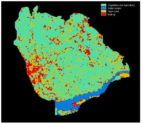
Landsat MSS for 1973 and Landsat TM for 1987 of 70 m spatial resolution was used for analysing urban sprawl. The remote sensing data corresponding to Landsat MSS for 1973 was obtained from the Earth Science Data Interface (ESDI) of the Global Land Cover Facility (GLCF), University of Maryland and NASA. The Landsat TM data for 1987 was procured from the National Remote Sensing Agency (NRSA), Hyderabad. The multi-spectral data was analysed using IDRISI 32 (http://www.clarklabs.org). The image analyses included band extraction, restoration, FCC generation, enhancement and classification. Training data was obtained in the field using the GPS and accordingly training polygons were created along with corresponding attribute data, which was later verified with the composite image. Based on these signatures, corresponding to various land features, image classification was done using Gaussian Maximum Likelihood Classifier. The classified image showing the built-up of 1973 and 1987 are given in Figure 4.5 and 4.6.
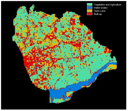
Area under built-up theme was recognized and extracted from the imagery and the area for 1973-1987 was computed. By overlaying the village/ward boundaries, village/ward-wise land use details were obtained. The distribution of village-wise land use of the study area for 1973 and 1987 are given in Figures 4.7 and 4.8 respectively.
Figure 4.7: Land Use of Mangalore Region in 1973
Figure 4.8: Land Use of Mangalore Region in 1987
The corresponding land use change in the region with respect to each of the land use classes are shown in Figure 4.9.
Figure 4.9: Land Use Change in Mangalore Region from 1973 to 1987
4 . 2 . 2 Population Growth and Buit-up Area |
From the analysis of the rates of development in the Mangalore region it was found that the amount of increase in built-up was nearly three times to that of the population growth. Thus, implying that even though the rate of population growth was around 50 %, the corresponding change in the built-up area was about 150 %. This indicated that more land was consumed per person, than what was being consumed earlier. The change in population in the region was found to be 70706 in 1987 as against 47424 in 1973, thereby attributing a percentage change of 49.09 %. However, when the built-up area was computed for the same duration, it was found that the built-up area had increased from 5.3473 sq. km to 13.5595 sq. km attributing almost 153.57 % change from 1973 to 1987 (Table 4.1). In sum, it indicated that for every increase in population by 1 %, the built-up increase was almost 3 %.
Table 4.1: Percentage Change of Built-up Area, Population, and Built-up Density from 1972 to 1987
Study Area |
1973 |
1987 |
Percentage Change |
Built-up Area (sq. km) |
5.3473 |
13.5595 |
153.57 % |
Population |
47424 |
70706 |
49.09 % |
Built-up Density |
0.09054 |
0.22871 |
152.60 % |
The per capita land consumption refers to utilization of all land for infrastructure and development activities like the commercial, industrial, educational, and recreational establishments along with the residential establishments per person. Since most of the activities pave way for employment and livelihoods, the development of land is seen as a direct consequence of region's economic development and hence it can be concluded that the per capita land consumption is inclusive of all the associated land development.
4.2.3 Modelling Urban Sprawl |
The land use analysis of the region and the preliminary analysis on the population growth for the same time period as discussed in the previous section indicated some significant relationships with the change of built-up area to the population growth, and the population-built-up density. Population has been for long accepted as a key factor of urban sprawl. The spatial organization of the built-up area can be obtained by computing the Entropy for the built-up density. Yeh and Li (2001) and Sudhira et al. (2003) have documented the application of entropy in urban sprawl studies. Further, the urban sprawl phenomenon is influenced by the distance of the land from the city centre as evinced from following regressions model.
Application of regression techniques for analyzing urban growth has been attempted for establishing the relationships between urban growth and its drivers. Cheng and Masser (2003) report the spatial logistic regression technique used for analysing the urban growth pattern and subsequently model the same for a city in China. Sudhira et al. (2004b) also report the multivariate linear regression technique for analyzing the urban sprawl. In order to quantify and test for relationships with respect to the urban sprawl, the different drivers, which were considered for regression analyses, were:
Initially, various regression analyses (linear, quadratic, exponential and logarithmic) were carried out to ascertain the nature of significance of the causal factors (independent variables) on the sprawl, quantified in terms of built-up. The linear, quadratic (order = 2), and logarithmic (power law) regression analyses were tried. All these regression analyses revealed the individual contribution by the causal factors on the sprawl. However, to assess the cumulative effects of causal factors, stepwise regression analysis considering multivariate was done. In the multivariate regression it is assumed that the relationship between variables is linear. The multivariate regression gives the cumulative relationship among the variables.
In order to explore the probable relationship of built-up (dependent variable) with causal factors of sprawl (population change, built-up density, entropy, etc.), multi-variable regression analyses were carried out to assess the cumulative effect of causal factors. The multivariate regression analyses reveal that all causal factors have a significant role in the sprawl phenomenon. The probable relationship for the built-up in subsequent year was:
Built-up = 0.08353 * Population Change + 24.3115 * Built-up1/VillageArea + 0.23898 * Entropy - 0.21114 * Mangalore Distance - 0.2153 Equation 4
r = 0.9664; p < 0.01; SE y estímate = 0.5224
4.2.4 Prediction of Urban Sprawl |
It is evident form the above relationship that the subsequent built-up has a significant relation with the drivers identified. Subsequently, the likely increase in the built-up for each year up to 1999 was predicted using the Equation 4. For example, to project built-up for 1999, corresponding population was computed considering annual growth rate based on the historical population data of 1961-2001 and the same was used in the equation to obtain the built-up area for the corresponding year.
The built-up area so obtained established the demand on land for conversion into built-up every year. This demand is utilized in the transition rules of the CA to allocate the land use into built-up in the subsequent years based on the suitability and constraints.
4.2.5 Mult-criteria Evalution for Land Suitability |
White et al., (1997) suggest the utility of assigning suitability of any cell for being allocated into built-up in the CA transitional rules. This concept has also been subsequently applied in various other CA models (Singh, 2003; Sun, 2003). On the similar lines, the multi-criteria evaluation was carried out for evaluating suitability of land cover to be allocated into built-up. The availability of suitable land is another prime factor for urban sprawl. The chief land use / land cover classification carried out for the satellite imagery includes, already developed (built-up) area, water bodies (sea, rivers, streams, tanks, lakes, etc), area under vegetation (agriculture, plantation, paddy, etc) and area under open land (barren, uncultivated, unused open land). The themes of already developed areas and water bodies' act as constraints for any further development. However, the probability of open land, barren land and uncultivated land for future built-up is very high. Similarly the possibility of area under vegetation to be converted into built-up as a result of sprawl cannot be ruled out. Apart from the prevalent land cover classes, the distances from the city centre and the roads are other important factors. Closer the distances from the city centre and the roads, the land has higher probability of becoming developed. Thus a sigmoidal monotonically decreasing fuzzy membership is assigned to weigh the factors of road and city centre distances.
Thus, each of the factors is evaluated for the suitability based on the criterion to each of the factor. As in the case of ordered weighted averaging, the suitability is defined by:
Equation 5 |
where, S = suitability; w i = weight of factor i (and sum of the factor weights = 1) ; and x i = criterion score of factor
The key factors and constraints considered are given in Table 4.2. Thus, a final suitability image is obtained wherein each cell has the suitability value based on the above factors and constraints defined.
Table 4 . 2 : Factors and Constraints
Factors |
Land Use: Open land |
Constraints |
Built-up |
From the suitability images so obtained, the image is ranked according to the probability that which cells are having the higher probability to be converted from other land use classes into built-up.
4.2.6 The CA Transition Rules |
The CA transitions are defined for the allocation of new built-up into other land use classes. The allocation is determined by the demand established by the statistical model. Further the allocation is also based on the suitability of the cells which area ranked after the multi-criteria evaluation for the suitability of the land. In one-iteration of the CA model, the simulation time is set to one year and so the model would allocate the land use into urban for the amount determined by the prediction model for demand also established for one-year simulation time. An underlying assumption is that only those land use classes other than urban would be considered for new urban areas implying that the urban growth will only increase and would never recede. Thus, when the simulation is executed, a set of output for the respective years would be depicting the future urban growth.
Thus the CA model for simulating urban growth is configured for the area under study by considering some of the drivers. With the basis of such a CA model, it can be seen that although the model can simulate for the future scenarios, the model is yet incapable of directly interacting with the drivers dynamically. For example, in the event that there is a sudden upsurge in population in one of the regions, the present configured model is incapable of addressing such scenarios. The transition rules of the CA model, so defined are inept to reflect the dynamic changes of the drivers by not interacting with them directly. Further the transition rules are system wide and so much of the details are generalized in the over all model. In order to address these inabilities of the CA model, the utility of the agent-based models in these scenarios is the crux of the research.
4.3 Agent-based Models in Simulating Urban Sprawl |
In view of the above-mentioned shortcomings of the CA based models, the integration of agent-based models is attempted in this research to demonstrate that the agent-based models can act a synthetic interface to the dynamic drivers of the system and the simulation framework. Noting the key characteristics of the agent-hood, that they are autonomous, have social ability, are responsiveness, and pro-active, the same is infused into the framework discussed in the previous chapter. These agents are conceived to diffuse into the CA model and initiate transitions, respond, exchange and report accordingly to the properties associated with each of the agent-based models. Such properties are essential for these agents to facilitate the human-decision making involved in the simulation in more realistic sense. Thus agents of an agent-based model to initiate transitions would diffuse into the CA transition to enact such functions. Likewise, agents of those agent-based models to respond or react would act accordingly. On the similar lines, the agents can be conceived to represent the realistic decision-making undertaken apart from interacting with the drivers dynamically. The interactions among the drivers by these agents are simulated by means of a feedback loops with the CA transitions. The agent manifestations into the CA transition rule resulting the final transitions based on the feedback loops is as shown in Figure 4.11. The feedback loops are associated with the different agents and their behaviours for which they are modelled. Subsequently, the final transition rule gets the update from these agents before updating the cell state in the subsequent iterations apart from the inherent CA transition rules.
Figure 4.10: Feedback Loops between CA Transitions and Agent-based State Transitions enabling the Final State Transitions
An essential aspect to be addressed involving these feedback loops in a geo-spatial discrete-time models is the capabilities of these different models to represent the dynamics and respond to them at the respective spatial and temporal scales of the models. In sum, within the dynamics of urban sprawl, there are so many drivers that are system-wide and specific to certain localities, implying the variation in scales of their activity in both space and time. Each of the agent-based models representing the drivers is considered as a discrete-time stepped models, while the general CA being another discrete-time stepped model with similar time advancement mechanisms. Thus, while dealing with these different space and time variant models adequate care has to be ensured for the synchronization of such models. And so, for the current simulation, the framework developed and discussed in Chapter 3 is used to ensure the applicability of the agent-based cellular automata systems.
4.3.1 Agents in the Simulation Framework |
Specific agent-based models are conceived for the use case of simulating the dynamics of urban sprawl. Among the key factors responsible for the dynamics of urban sprawl is the population of the region. In such case, the population development process can be considered as an agent that is driving the sprawl phenomenon. In the conceptualised CA model (Figure 4.4), even though the population of the region under investigation is considered, the model is not so dynamic enough to accommodate for any change in the population already fed in the model to be reflected in the CA transitions. Further, the population considered for the conceptualised CA model is computed annually based on the growth rates of the previous years. In spite of a built-up prediction model established to reflect the population of the villages in the study area, the typical CA model does not facilitate any interaction of these drivers. Consequently, the idea is to utilize the properties of the agent-based models as the representation of these drivers so that they can better reflect these properties.
Apart from the population development process driving the sprawl, the other drivers can be the infrastructure initiatives. The infrastructure initiative can be considered as an addition of a ring road around the city or demarcation of an area under different land cover as a residential layout. Such infrastructure initiatives are very typical in the fast and rapidly growing cities like Mangalore, also common in most of the similar cities of the country. The agent-based model conceived here representing the infrastructure initiative is for the ring road development process. In the typical instances of the ring road development around a city, the actual construction of the roads takes about two to three years. By the time the ring road is near completion, other allied developments like the establishments of institutions, industries, residential layouts in the vicinity are all imminent. Thus, an over all implication of such initiative in the due course of time, say about five years from the completion of the ring road, the region in the vicinity of the ring road will be more or less developed or the land use will be converted into urban. This above scenario is of an infrastructure initiative is conceptualised as an agent-based model which has multiple events resulting out of such activity and the pattern of growth varying over time. The initial creation of a ring road, which can be thought of as an addition of a poly-line feature around the city, results in the suitability of the land becoming into built-up with the completion of the ring road. Thus, the features (land use class) surrounding the poly-line (ring road), gets a higher suitability values over a period of three years also based on the prevalent land use classes and constraints. Eventually, all the land use classes surrounding the new ring road would become urban, subject to the constraints of the system. This process itself can represent one such agent-based model to initiate state transitions over time depending on the situations in relation to the prevalent conditions. In the same situation, different agents can also be defined to report the nature of growth taking place over time. With the possibility of defining all these processes as agent-based models, the agent-automata described for this scenario over a specific period of time, can be coupled in over all simulation, which would enable in the visualization of such what if' scenarios more effectively. The utility of involving the agents in the simulation of urban sprawl can be thought of as much as those only limited by the conceptualisation of the modeller and other resource constraints.
In this research the general scheme for building the agents in the geo-spatial domain suggested is discussed in the foregoing section while the implementation of the same is taken up in the next chapter. An alternate way of introducing the agents in the geo-spatial domain would be to enable the prevalent tools for agent-based modelling like the NetLogo, StarLogo, SWARM, etc. to interact with the geo-spatial domain. This may be achieved by programming these tools to communicate and exchange the geo-spatial data with appropriate interfaces within the simulation framework of the respective agent-based modelling tools.
4.3.2 Agents in Geo-Spatial Domain |
In light of the above discussion of involving the agents in the geo-spatial domain, it becomes consequential that the spatial relationships or the topologies and specific geometry to these agents are defined so that they can be enabled to act in conjunction with the CA model. An ensuing approach in this regard was the creation of an interface for building the agents as geographic features, such as point, poly-line or a polygon thereby defining the spatial extents of these. The scheme of activity for such utility is as shown in Figure 4.11. In the next step the temporal dimension is attached to these agent-features so defined within the interface. Subsequently, the agent-behaviour in question or the model for the agent activity is established. Thus each of the agent-based models conceived for the region under investigation can be created on the fly before the simulation is executed. However, the agents are until now represented as geographic features, need to be acting in the cellular space, for which these agent-features are rasterised at appropriate scales. The scales at which they are rasterised needs to be calibrated so as to ensure effective synchronization and represent the realistic behaviour of the system in question. This interface to build agents along with their extents, duration and defining the behaviour is to act in concurrence with the geo-spatial data representing the different land use classes.
Figure 4.11: Scheme for Agent-building in Geo-spatial Domain
Each of the agent-based models thus defined are treated as one discrete time-stepped simulation system. The behaviour of different agent-automata over the simulation time is shown in Figure 2.2. The imminent task for ensuring the simulations is by properly scheduling the different models based on the spatial extents and synchronizing these time-variant models appropriately in the overall framework.