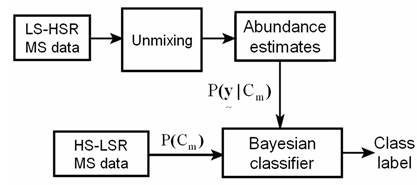
Figure 11: Hybrid Bayesian Classifier.

In the following section, linear unmixing using Orthogonal Subspace Projection (OSP) and Bayesian classifier are discussed. Next, HBC is discussed with experimental results and validation.

6.1       Linear unmixing: With M spectral bands and N classes (C1,..,CN), each pixel has an associated M-dimensional pixel vector  whose components are the pixel intensities corresponding to the M spectral bands. Let , where, for ,  is a  column vector representing the endmember spectral signature of the nth target material. For a pixel, let  denote the fraction of the nth target material signature, and  denote the N-dimensional abundance column vector. The linear mixture model for  is given by

                                                                                                                                                               (21)

where, , are i.i.d.  (Kumar et al., 2008). Equation (19) represents a standard signal detection model where  is a desired signal vector to be detected. Since, OSP detects one target at a time, we divide a set of N targets into desired  and undesired  targets. A logical approach is to eliminate the effects of undesired targets that are considered as “impeders” to  before detecting. To estimate, the desired target material is . The term  in (21) can be rewritten to separate the desired spectral signature :

                                                                                                                                             (22)                              
where  and . Thus the interfering signatures in  can be removed by the operator,

                                                                                                                                        (23)

which is used to project  into a space orthogonal to the space spanned by the interfering spectral signatures, where  is the  identity matrix (Change, 2005). Operating on  with , and noting that ,

.                                                                                                                                                 (24)

After maximizing the SNR, an optimal estimate of  is

                                                                                                                                              (25)

Note that  and thus  can be taken as proportional probabilities of the N classes i.e. .

6.2       Bayesian classifier: Associated with any pixel, there is an observation . With N classes , Bayesian classifier calculates the posterior probability of each class conditioned on  (Han and Kamber):

                                                                                                                                          (26)

In (26), since  is constant for all classes, only  is considered.  is computed assuming class conditional independence, so,  is given by                    (27)

LISS-III MS classified image using conventional Bayesian classifier is shown in figure 12 (a). Assuming that there are six (fixed) number of representative endmembers (pure pixels), the entire image was modeled in terms of those spectral components, extracted using N-FINDR algorithm (Winter, 1999) from MODIS images. In the absence of pure pixels, alternative algorithms (Plaza et al., 2004) can be used for endmember extraction, which is a limitation of N-FINDR. It may be noted that some objects (for example buildings with concrete roofs, tiled roofs, asphalt, etc.) exhibit high degrees of spectral heterogeneity representing variable endmembers. This intra-class spectral variation with variable endmembers can be addressed through techniques discussed in (Bateson et al., 2000; Song, 2005; Foody and Doan, 2007). 

Abundance values were estimated for each pixel through unmixing and used as prior probabilities in HBC to classify LISS-III MS data (Fig. 12 (b)). Table 11 is the class statistics and table 12 indicates the producer’s and user’s accuracies. The overall accuracy and Kappa for HBC (93.54%, 0.91) is higher than Bayesian classifier (87.55%, 0.85). For any particular class, if the reference data has more pixels with correct label, the producer’s accuracy is higher and if the pixels with the incorrect label in classification result is less, its user’s accuracy is higher (Mingguo et al., 2009). Bayesian classifier wrongly classified many pixels belonging to waste/barren/fallow as builtup. Forest class was over-estimated and plantation was under-estimated by Bayesian classifier. The only minority class in the study area is water bodies. Classified image using conventional Bayesian classifier had 1.08% (8854 ha) of water bodies in the study area. After the ground visit, we found that there are not many water bodies and the extents of most individuals were < 2000m2. Therefore, only a few water bodies that had spatial extent ≥ 62500 m2, could be used as endmembers. The minimum detected water class was 5% using unmixing of LS-HSR data. It may have happened that the prior probability was unlikely for this class while classifying the LISS-III MS data using HBC. The classified image obtained from HBC showed 0.81% (66.20 ha) of water bodies. A few pixels were wrongly classified using HBC, therefore, the producer’s accuracy decreased from 90.91 (in conventional Bayesian classifier) to 88.18% (in HBC).

Figure 12: LISS-III MS classified images: (a) Bayesian classifier, (b) HBC.

Table 11: Class statistics from Bayesian and HBC for LISS-III data

Classifiers →	Bayesian classifier		HFC
Class ↓	Ha	%	Ha	%
Agriculture	155, 451	19.04	142931	17.51
Builtup	139, 759	17.12	79280	9.71
Forest	93, 241	11.42	55721	6.83
Plantation	89,493	10.96	176132	21.58
Waste land	329, 473	40.36	355587	43.56
Water bodies	8854	1.08	66.20	0.81

 

Table 12: Accuracy assessment for LISS-III data

Classifiers →	Bayesian classifier		HBC
Class ↓	PA*	UA*	PA*		UA*
Agriculture	87.54	87.47	90.15	↑	95.56	↑
Builtup	85.11	81.68	89.39	↑	98.33	↑
Forest	85.71	88.73	92.61	↑	96.36	↑
Plantation	84.44	91.73	95.95	↑	91.03	↓
Waste land	88.03	90.37	98.67	↑	89.66	↓
Water bodies	90.91	88.89	88.18	↓	97.00	↑
Average	86.96	88.15	92.49	↑	94.66	↑

     * PA – Producer’s Accuracy; UA – User’s Accuracy.

However, given the same set of training pixels for classification, the user’s accuracy has increased from 88.89 to 97%. Producer’s accuracy increased for agriculture (2.6%), builtup (4.3%), forest (7%), plantation (11.5%) and waste land (10.6%) and user’s accuracy increased for agriculture (8%), builtup (16.6%), forest (7.6%) and water bodies (8%) in HBC output. On the other hand, producer’s accuracy decreased (2.7%) for water bodies and user’s accuracy decreased (~0.7%) for plantation and waste land classes in agreement with the similar observations reported in Mingguo et al. (2009). HBC was intended to improve classification accuracies by correctly classifying pixels which were likely to be misclassified by Bayesian classifier. Therefore a cross comparison of the two classified images located the pixels that were assigned different class labels at the same location. These wrongly classified pixels when validated with ground data revealed a 6% (~1742832 pixels) improvement in classification by HBC.

In the second experiment, IKONOS MS data (4 bands of 4 m, acquired on November 24, 2004) of 700 x 700 size and Landsat ETM+ data (6 bands excluding Thermal and Panchromatic, of 30m, acquired on November 22, 2004) of 100 x 100 dimension were co-registered (RMSE - 0.09). Landsat pixels were resampled to 28 m so that 49 IKONOS pixels would fit in 1 Landsat pixel. The scenes correspond to Bangalore city, India near the central business district having race course, bus stand, railway lines, parks, builtup with concrete roofs, asbestos roofs, blue plastic roofs, coal tarred roads with flyovers and a few open areas (playground, walk ways, vacant land, etc.). Class proportions from Landsat image pixels were used as prior probabilities to classify the IKONOS MS images using HBC (Figure 13 (b)). The overall accuracy and Kappa for HBC (89.53%, 0.87) is higher than Bayesian classifier (80.46%, 0.69). Producer’s accuracy increased by 17% for concrete, asbestos, blue plastic roof and open area and decreased by 7% for vegetation in HBC (table 14). User’s accuracy increased by ~5.5% for all the classes in HBC. Bayesian classifier wrongly classified and overestimated many pixels belonging to open area as asbestos roof (table 13). Vegetation was overestimated by 9% using Bayesian classifier and open area was underestimated by ~15%. A cross comparison of the two classified images showed that 95733 pixels (0.33% of the study area) were differently classified by the two classifiers. Validation of these pixels showed an improvement of 9% by HBC, higher than accuracies reported in (Janssen and Middelkoop, 1992; Cetin et al., 1993; Strahler, 1980).

Table 13: Class statistics for IKONOS data

Classifiers →	Bayesian classifier		HBC
Class ↓	Ha	%	Ha	%
Concrete roof	346.67	44.34	356.18	45.56
Asbestos roof	47.99	7.41	6.79	0.87
Blue plastic roof	5.83	0.75	0.21	0.03
Vegetation	329.72	42.18	260.01	33.26
Open area	41.60	5.32	158.58	20.28

 

 

 

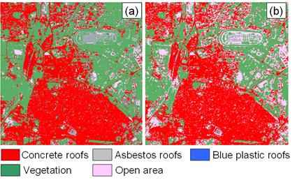
Figure 13: IKONOS classified images: (a) Bayesian classifier, (b) HBC.

 

Table 14: Accuracy assessment for IKONOS data                           

Classifiers →	Bayesian classifier		HBC
Class ↓	PA	UA	PA		UA
Concrete roofs	69.99	84.01	76.49	↑	93.89	↑
Asbestos roofs	84.77	87.77	91.89	↑	94.46	↑
Vegetation	94.21	87.55	87.24	↓	89.13	↑
Blue plastic roof	84.33	81.17	97.00	↑	85.60	↑
Open area	51.49	69.49	95.00	↑	74.22	↑
Average	76.96	81.99	89.52	↑	87.46	↑