Algorithm implimentation
KONOS MS
Figure 4 is the high resolution Google Earth image and figure 5 is the false colour composite (FCC) of IKONOS 4 MS bands (700 rows x 700 columns) corresponding to Bangalore City, India. The part of the city shown in scene is highly urbanised with the central business district. It consists of highly contrasting and heterogeneous features such as race course (as oval shape in the first quadrant of the image), bus stand with semi-circular platforms, railway station with railway lines in the second quadrant, a park below the race course, dense builtup with concrete roofs, and some buildings with asbestos roofs, blue plastic roofs (one in the vicinity of the race course and two near the railway lines), tarred roads with flyovers, vegetation and few open areas (such as a playground, walk ways and vacant land).
For DT, set of rules were extracted using See5 (http://www.rulequest.com) with 25% global pruning. These rules were then used to classify IKONOS MS data. For KNN, number of nearest neighbour was kept 1 in feature space. In case of conflict, random allocation to LU class was done. In NN based classification, a logistic function was used along with 1 hidden layer. Output activation threshold was set to 0.001, training momentum was set to 0.1, training RMS exit criteria were set to 0.1, training threshold contribution was 0.1, and the training rate was maintained at 0.2 to achieve the convergence at 465 iterations (figure 6). KNN and NN algorithms were coded in C programming language in Linux. RF was implemented using a random forest package (Liaw and Weiner, 2002), available in R interface (http://www.r-project.org). SMAP was implemented through free and open source GRASS GIS (http://wgbis.ces.iisc.ac.in/grass). SVM was implemented using both polynomial and RBF using libsvm package (http://www.csie.ntu.edu.tw/~cjlin/libsvm/). A second degree polynomial kernel was used with 1 as bias in kernel function, gamma as 0.25 (usually taken as 1 divided by the number of input bands), and penalty as 1. For RBF, gamma was 0.25 and penalty parameter was set to 1.
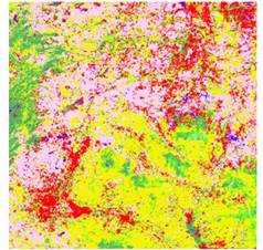
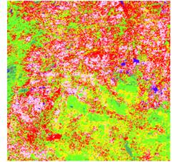
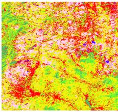
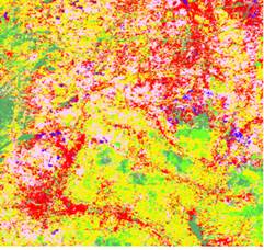
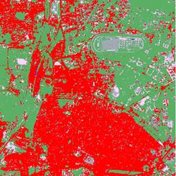
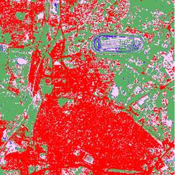
Classified images of IKONOS data are shown in figure 7. The class statistics are as listed in table 2 and table 3 gives the accuracy assessment with highest 4 overall accuracies highlighted in bold.
Table 2: LU estimates from IKONOS MS using advanced classifiers
Classes → |
Concrete
roof |
Asbestos roof |
Blue plastic
roof |
Vegetation
(parks, garden) |
Open area
(play ground) |
Algorithms↓ |
ha |
% |
ha |
% |
ha |
% |
ha |
% |
ha |
% |
MLC |
346.67 |
44.34 |
47.99 |
7.41 |
5.83 |
0.75 |
329.72 |
42.18 |
41.60 |
5.32 |
DT |
344.36 |
44.05 |
16.87 |
2.16 |
1.86 |
0.24 |
259.36 |
33.18 |
159.31 |
20.38 |
KNN |
342.64 |
43.83 |
11.77 |
1.51 |
11.91 |
1.52 |
268.71 |
34.37 |
146.73 |
18.77 |
NN |
381.77 |
48.83 |
7.69 |
0.98 |
- |
- |
280.17 |
35.84 |
112.12 |
14.34 |
RF |
351.74 |
44.99 |
9.53 |
1.22 |
1.88 |
0.24 |
260 |
33.26 |
158.61 |
20.29 |
SMAP |
386.36 |
49.42 |
4.59 |
0.59 |
0.52 |
0.07 |
231.71 |
29.64 |
158.58 |
20.28 |
SVM (Polynom) |
361.84 |
46.28 |
4.37 |
0.56 |
27.34 |
3.50 |
246.02 |
31.47 |
142.20 |
18.19 |
SVM (RBF) |
352.83 |
45.13 |
4.29 |
0.55 |
21.21 |
2.71 |
247.38 |
31.64 |
156.04 |
19.96 |
Total |
781.76 (ha) |
100 % |
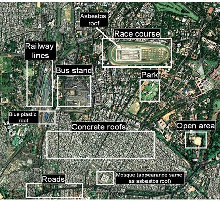
Figure 4: Google Earth image corresponding to the IKONOS image.
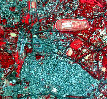
Figure 5: FCC of the IKONOS image.
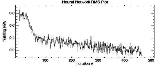
Figure 6: Plot of training RMS versus iterations of NN.
Figure 7: Classification of IKONOS MS data through advanced classification techniques.
Table 3: Accuracy assessment for IKONOS classified data
Algorithm |
Class |
Producer’s Accuracy (%) |
User’s Accuracy (%) |
Overall Accuracy (%) |
Kappa |
MLC |
Concrete |
69.99 |
84.01 |
80.46 |
0.6900 |
Asbestos |
84.77 |
87.77 |
Blue Plastic |
84.33 |
81.17 |
Vegetation |
94.21 |
87.55 |
Open area |
51.49 |
69.49 |
|
|
|
|
|
|
DT |
Concrete |
84.74 |
81.00 |
82.22 |
0.8025 |
Asbestos |
83.75 |
79.00 |
Blue Plastic |
84.74 |
80.00 |
Vegetation |
82.00 |
87.00 |
Open area |
76.92 |
83.00 |
|
|
|
|
|
|
KNN |
Concrete |
95.35 |
95.00 |
79.85 |
0.7150 |
Asbestos |
81.23 |
75.00 |
Blue Plastic |
80.00 |
79.00 |
Vegetation |
50.00 |
75.00 |
Open area |
91.00 |
76.92 |
|
|
|
|
|
|
NN |
Concrete |
52.63 |
68.50 |
69.84 |
0.6125 |
Asbestos |
90.91 |
50.00 |
Blue Plastic |
73.33 |
71.00 |
Vegetation |
71.43 |
63.00 |
Open area |
82.61 |
75.00 |
|
|
|
|
|
|
RF |
Concrete |
92.50 |
89.99 |
85.25 |
0.8250 |
Asbestos |
89.15 |
81.00 |
Blue Plastic |
85.00 |
87.00 |
Vegetation |
85.00 |
83.00 |
Open area |
76.92 |
83.00 |
|
|
|
|
|
|
SMAP |
Concrete |
87.21 |
88.76 |
86.92 |
0.8475 |
Asbestos |
89.29 |
83.00 |
Blue Plastic |
91.11 |
88.00 |
Vegetation |
91.00 |
89.00 |
Open area |
76.92 |
85.00 |
|
|
|
|
|
|
SVM (Polynomial) |
Concrete |
89.67 |
55.00 |
79.97 |
0.7125 |
Asbestos |
81.33 |
60.00 |
Blue Plastic |
91.74 |
85.00 |
Vegetation |
95.33 |
91.00 |
Open area |
70.64 |
80.00 |
|
|
|
|
|
|
SVM
(RBF) |
Concrete |
89.67 |
55.00 |
79.97 |
0.7125 |
Asbestos |
81.33 |
60.00 |
Blue Plastic |
91.74 |
85.00 |
Vegetation |
95.33 |
91.00 |
Open area |
70.64 |
80.00 |
IRS LISS-III MS
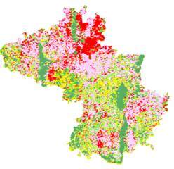
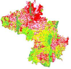
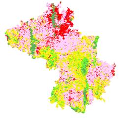
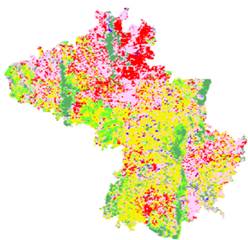
LISS-III MS of 23.5 m x 23.5 m spatial resolution (as shown in FCC in the first image in figure 8 – LISS-III FCC) represents a portion of Kolar district, north of new Bangalore International Airport, India. Training and testing data were collected separately for agriculture, builtup, evergreen/semi-evergreen forest, plantations/orchards, wasteland/barren/rock and water bodies. Classified image using the seven algorithms are shown in figure 8. LU statistics are given in table 4 and highest 4 overall accuracy are highlighted in bold in table 5.
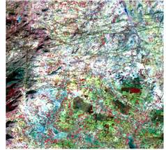
LISS-III FCC
|
 MLC MLC
|
 DT DT
|
 KNN KNN
|
 NN NN
|
 RF RF
|
 SMAP SMAP
|
 SVM (Polynomial) SVM (Polynomial)
|
 SVM (RBF) SVM (RBF)
|

|
Figure 8: Classification of IRS LISS-III MS data through advanced classification techniques
Table 4: LU estimates from IRS LISS-III MS using advanced classifiers
Classes → |
Agriculture |
Built up |
Forest |
Plantation |
Wasteland |
Water bodies |
Algorithms↓ |
ha |
% |
ha |
% |
ha |
% |
ha |
% |
ha |
% |
ha |
% |
MLC |
15388 |
32.32 |
7524 |
15.80 |
4091 |
8.59 |
4951 |
10.40 |
15184 |
31.89 |
473.13 |
0.99 |
DT |
10510 |
21.94 |
13923 |
29.07 |
1307 |
2.73 |
12210 |
25.49 |
9467 |
19.76 |
483.57 |
1.01 |
KNN |
20447 |
42.69 |
10109 |
21.10 |
2320 |
4.84 |
5993 |
12.51 |
8797 |
18.37 |
235.95 |
0.49 |
NN |
18455 |
38.53 |
9856 |
20.58 |
3619 |
7.56 |
3298 |
6.88 |
12082 |
25.22 |
591.34 |
1.23 |
RF |
16016 |
33.44 |
12916 |
26.96 |
2492 |
5.20 |
5973 |
12.47 |
9990 |
20.85 |
514.52 |
1.07 |
SMAP |
19431 |
40.56 |
4279 |
6.93 |
1029 |
2.15 |
4968 |
10.37 |
18057 |
37.70 |
137.72 |
0.29 |
SVM (Poly) |
14360 |
29.87 |
11830 |
24.70 |
1227 |
2.56 |
4862 |
10.15 |
15610 |
32.59 |
66.72 |
0.14 |
SVM (RBF) |
20071 |
41.9 |
6571 |
13.72 |
2709 |
5.65 |
7860 |
16.41 |
10488 |
21.89 |
203.3 |
0.42 |
Total |
47901.00 (ha) |
100% |
Table 5: Accuracy assessment for IRS LISS-III classified data
Algorithm |
Class |
Producer’s Accuracy (%) |
User’s Accuracy (%) |
Overall Accuracy (%) |
Kappa |
MLC |
Agriculture |
91.21 |
93.87 |
86.59 |
0.8323 |
Builtup |
88.33 |
89.33 |
Forest |
94.80 |
86.24 |
Plantation |
88.86 |
85.46 |
Wasteland |
85.20 |
82.81 |
Water bodies |
68.52 |
85.10 |
|
|
|
|
|
|
DT |
Agriculture |
94.72 |
57.47 |
75.89 |
0.7148 |
Builtup |
63.04 |
83.60 |
Forest |
93.87 |
70.38 |
Plantation |
95.75 |
76.15 |
Wasteland |
56.91 |
78.37 |
Water bodies |
76.38 |
67.00 |
|
|
|
|
|
|
KNN |
Agriculture |
89.36 |
89.44 |
89.02 |
0.8604 |
Builtup |
87.54 |
95.66 |
Forest |
94.90 |
87.99 |
Plantation |
89.00 |
88.00 |
Wasteland |
85.01 |
82.32 |
Water bodies |
85.18 |
94.00 |
|
|
|
|
|
|
NN |
Agriculture |
92.56 |
81.45 |
83.66 |
0.8112 |
Builtup |
81.30 |
91.63 |
Forest |
87.90 |
88.34 |
Plantation |
83.00 |
81.00 |
Wasteland |
74.42 |
81.56 |
Water bodies |
78.83 |
82.00 |
|
|
|
|
|
|
RF |
Agriculture |
93.96 |
74.73 |
82.29
|
0.7638 |
Builtup |
67.51 |
83.65 |
Forest |
91.57 |
85.70 |
Plantation |
80.00 |
81.00 |
Wasteland |
73.47 |
84.87 |
Water bodies |
85.09 |
86.00 |
|
|
|
|
|
|
SMAP |
Agriculture |
91.17 |
62.46 |
76.17 |
0.7365 |
Builtup |
79.49 |
64.98 |
Forest |
73.23 |
87.84 |
Plantation |
75.00 |
81.00 |
Wasteland |
51.15 |
72.56 |
Water bodies |
88.18 |
87.00 |
|
|
|
|
|
|
SVM (Polynomial) |
Agriculture |
75.28 |
48.04 |
68.83 |
0.6647 |
Builtup |
33.63 |
50.17 |
Forest |
90.55 |
84.49 |
Plantation |
64.00 |
68.00 |
Wasteland |
53.71 |
92.73 |
Water bodies |
69.35 |
96.00 |
|
|
|
|
|
|
SVM
(RBF) |
Agriculture |
90.49 |
85.83 |
88.18 |
0.8534 |
Builtup |
85.54 |
89.33 |
Forest |
90.90 |
86.69 |
Plantation |
93.14 |
87.15 |
Wasteland |
82.46 |
85.51 |
Water bodies |
90.17 |
91.00 |
Landsat ETM+ MS
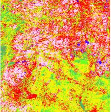
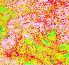
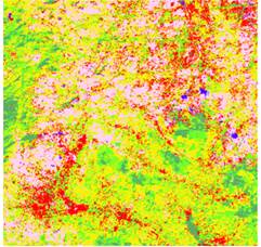
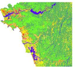
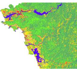
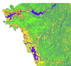
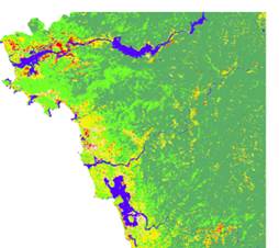
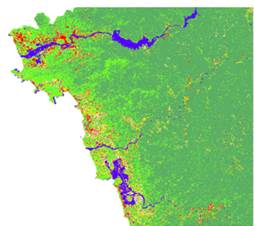
Landsat ETM+ MS data of Uttara Kannada district, Karnataka state, India and part of Western Ghats, India (first image in figure 9 is Google Earth image) were used for classification. Band 1 to 5 and band 7 of 2000 x 2000 size were classified using training data collected from field and validated using separate test data. The classified images using the seven techniques are shown in figure 9. Table 6 and 7 gives the LU statistics and accuracy assessment with highest 4 accuracies highlighted in bold.
Table 6: LU estimates from ETM+ using advanced classifiers
Classes → |
Agriculture |
Builtup |
Forest |
Plantation |
Wasteland |
Water bodies |
Algorithms↓ |
ha |
% |
ha |
% |
ha |
% |
ha |
% |
ha |
% |
ha |
% |
MLC |
18824 |
5.80 |
6386 |
1.97 |
226695 |
69.88 |
54043 |
16.66 |
5322 |
1.64 |
13157 |
4.06 |
DT |
51617 |
15.91 |
6398 |
1.97 |
158049 |
48.72 |
83446 |
25.72 |
9411 |
2.90 |
15502 |
4.78 |
KNN |
48566 |
14.97 |
8663 |
2.67 |
195457 |
60.25 |
50793 |
15.66 |
7582 |
2.34 |
13361 |
4.12 |
NN |
39075 |
12.04 |
8068 |
2.49 |
151979 |
46.85 |
97686 |
30.11 |
10609 |
3.27 |
17005 |
5.24 |
RF |
41629 |
12.83 |
5732 |
1.77 |
194666 |
60.00 |
56483 |
17.41 |
10826 |
3.34 |
15121 |
4.66 |
SMAP |
35992 |
11.09 |
4249 |
1.34 |
201454 |
62.01 |
64034 |
19.74 |
4953 |
1.53 |
13739 |
4.24 |
SVM (Poly) |
19292 |
5.95 |
6385 |
1.97 |
226815 |
69.92 |
54024 |
16.65 |
5319 |
1.64 |
12548 |
3.87 |
SVM (RBF) |
37680 |
11.62 |
6421 |
1.98 |
193195 |
59.56 |
54437 |
16.78 |
5319 |
1.64 |
27331 |
8.43 |
Total |
324421.68 (ha) |
100% |
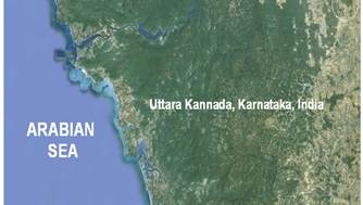 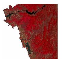 Google Earth image of UK, India ETM+ FCC Google Earth image of UK, India ETM+ FCC
|
|
 MLC MLC
|
 DT DT
|
|
 KNN KNN
|
 NN NN
|
|
 RF RF
|
 SMAP SMAP
|
|
 SVM (Polynomial) SVM (Polynomial)
|
 SVM (RBF) SVM (RBF)
|
|

|
|
Figure 9: Classification of ETM+ Plus data through advanced classification techniques.
Table 7: Accuracy assessment for ETM+ classified data
Algorithm |
Class |
Producer’s Accuracy (%) |
User’s Accuracy (%) |
Overall Accuracy (%) |
Kappa |
MLC |
Agriculture |
82.50 |
86.66 |
85.18 |
0.8190 |
Builtup |
84.00 |
85.00 |
Forest |
80.85 |
90.91 |
Plantation |
81.66 |
83.00 |
Wasteland |
83.00 |
89.67 |
Water bodies |
90.91 |
84.00 |
|
|
|
|
|
|
DT |
Agriculture |
83.33 |
86.67 |
84.54 |
0.7946 |
Builtup |
95.00 |
85.00 |
Forest |
82.63 |
80.61 |
Plantation |
85.75 |
80.00 |
Wasteland |
85.00 |
84.00 |
Water bodies |
83.33 |
83.21 |
|
|
|
|
|
|
KNN |
Agriculture |
84.41 |
87.00 |
86.98 |
0.8314 |
Builtup |
97.00 |
87.00 |
Forest |
76.43 |
89.79 |
Plantation |
87.45 |
86.67 |
Wasteland |
87.00 |
89.00 |
Water bodies |
87.00 |
85.00 |
|
|
|
|
|
|
NN |
Agriculture |
83.33 |
70.00 |
74.98 |
0.7142 |
Builtup |
85.00 |
82.00 |
Forest |
62.63 |
60.61 |
Plantation |
87.85 |
76.66 |
Wasteland |
77.00 |
71.00 |
Water bodies |
66.67 |
77.00 |
|
|
|
|
|
|
RF |
Agriculture |
87.44 |
86.66 |
83.37 |
0.7505 |
Builtup |
87.00 |
82.00 |
Forest |
74.26 |
81.82 |
Plantation |
82.57 |
84.73 |
Wasteland |
82.00 |
79.00 |
Water bodies |
90.91 |
82.00 |
|
|
|
|
|
|
SMAP |
Agriculture |
85.48 |
86.66 |
89.03 |
0.8596 |
Builtup |
98.00 |
99.00 |
Forest |
80.65 |
87.76 |
Plantation |
88.94 |
89.57 |
Wasteland |
89.00 |
87.00 |
Water bodies |
87.33 |
89.00 |
|
|
|
|
|
|
SVM (Polynomial) |
Agriculture |
87.27 |
80.00 |
85.35 |
0.8324 |
Builtup |
85.00 |
95.00 |
Forest |
88.70 |
81.82 |
Plantation |
81.66 |
85.47 |
Wasteland |
85.00 |
87.00 |
Water bodies |
85.55 |
81.67 |
|
|
|
|
|
|
SVM
(RBF) |
Agriculture |
76.25 |
83.33 |
83.77 |
0.7977 |
Builtup |
80.00 |
93.00 |
Forest |
80.85 |
80.91 |
Plantation |
81.66 |
83.33 |
Wasteland |
89.00 |
85.00 |
Water bodies |
90.91 |
81.00 |
MODIS
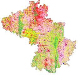
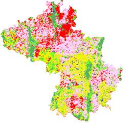
MODIS 8-day composite data (7 bands of 250 m x 250 m) were co-registered with known ground control points - GCPs (RMSE - 0.11) representing Kolar district in Karnataka having an area of 8238 sq. km. Training data (≥ 250 m x 250 m) were collected representing approximately 10% of the geographical area covering the entire spectral gradient of the classes. Separate test data were collected for validation. Preliminary survey revealed that there are six major LU classes in the study area – agriculture, builtup (urban/rural), evergreen/semi-evergreen forest, plantations/orchards, wasteland/barren rock/stony waste/sheet rock and water bodies/lakes/ponds/tanks/wetlands) that could constitute homogeneous MODIS pixels. Barren/rock/stone that have very limited ground area proportions and are unevenly scattered among the major six classes, were grouped under the wasteland category since they would form mixed pixels. The classified images are shown in figure 10 along with LU statistics (table 8) and accuracy assessment (in table 9).
 MODIS FCC MODIS FCC |
 MLC (IRS LISS-III MS) MLC (IRS LISS-III MS)
|
 MLC MLC
|
DT
|
 KNN KNN
|
 NN NN
|
 RF RF
|
 SMAP SMAP
|
 SVM (Polynomial) SVM (Polynomial)
|
 SVM (RBF) SVM (RBF)
|

|
Figure 10: Classification of MODIS data through advanced classification techniques.
Table 8: LU estimates from MODIS using advanced classifiers
Classes → |
Agriculture |
Builtup |
Forest |
Plantation |
Wasteland |
Water bodies |
Algorithms↓ |
ha |
% |
ha |
% |
ha |
% |
ha |
% |
ha |
% |
ha |
% |
MLC |
170247 |
20.68 |
130650 |
15.87 |
85352 |
10.37 |
107970 |
13.12 |
320767 |
38.57 |
8156 |
0.99 |
DT |
126752 |
15.92 |
133521 |
16.77 |
123061 |
15.46 |
93911 |
11.80 |
314126 |
39.46 |
4790 |
0.60 |
KNN |
1702834 |
20.69 |
142703 |
17.34 |
99731 |
12.12 |
99441 |
12.08 |
302091 |
36.70 |
8892 |
1.08 |
NN |
179720 |
21.83 |
217984 |
26.48 |
629012 |
7.64 |
160886 |
19.55 |
199462 |
24.23 |
2186 |
0.27 |
RF |
238517 |
28.99 |
97328 |
11.83 |
66366 |
8.07 |
54214 |
6.59 |
363934 |
44.23 |
2392 |
0.29 |
SMAP |
224464 |
27.27 |
117323 |
14.25 |
79338 |
9.64 |
83048 |
10.09 |
320813 |
37.76 |
8156 |
0.99 |
SVM (Poly) |
180567 |
21.94 |
215810 |
26.22 |
63072 |
7.66 |
161386 |
19.61 |
199785 |
24.28 |
2382 |
0.29 |
SVM (RBF) |
171020 |
20.80 |
127450 |
15.50 |
85565 |
10.41 |
108378 |
13.18 |
321455 |
39.11 |
8162 |
0.99 |
Total |
823141.42 (ha) |
100% |
Table 9: Accuracy assessment for MODIS classified data
Algorithm |
Class |
Producer’s Accuracy (%) |
User’s Accuracy (%) |
Overall Accuracy (%) |
Kappa |
MLC |
Agriculture |
93.70 |
70.26 |
70.43 |
0.6721 |
Builtup |
44.00 |
46.32 |
Forest |
80.00 |
66.22 |
Plantation |
65.90 |
77.88 |
Wasteland |
68.90 |
83.33 |
Water bodies |
70.75 |
75.38 |
|
|
|
|
|
|
DT |
Agriculture |
60.24 |
53.07 |
59.51 |
0.4860 |
Builtup |
58.06 |
63.00 |
Forest |
38.02 |
58.35 |
Plantation |
62.00 |
54.00 |
Wasteland |
65.19 |
63.28 |
Water bodies |
71.00 |
67.85 |
|
|
|
|
|
|
KNN |
Agriculture |
53.82 |
95.56 |
62.74 |
0.5801 |
Builtup |
48.90 |
44.33 |
Forest |
65.00 |
64.00 |
Plantation |
58.18 |
63.85 |
Wasteland |
71.31 |
45.86 |
Water bodies |
70.87 |
71.29 |
|
|
|
|
|
|
NN |
Agriculture |
54.44 |
76.08 |
64.14 |
0.5633 |
Builtup |
48.73 |
44.33 |
Forest |
64.00 |
63.87 |
Plantation |
83.04 |
75.39 |
Wasteland |
65.00 |
58.62 |
Water bodies |
68.76 |
67.44 |
|
|
|
|
|
|
RF |
Agriculture |
62.98 |
88.17 |
76.21 |
0.7357 |
Builtup |
59.44 |
54.33 |
Forest |
75.00 |
79.00 |
Plantation |
92.93 |
91.03 |
Wasteland |
83.17 |
72.41 |
Water bodies |
79.00 |
77.00 |
|
|
|
|
|
|
SMAP |
Agriculture |
67.26 |
71.69 |
69.44 |
0.6558 |
Builtup |
47.83 |
54.00 |
Forest |
82.54 |
75.43 |
Plantation |
61.70 |
65.72 |
Wasteland |
78.87 |
71.17 |
Water bodies |
81.47 |
75.56 |
|
|
|
|
|
|
SVM (Polynomial) |
Agriculture |
54.44 |
76.08 |
64.65 |
0.5633 |
Builtup |
48.73 |
44.33 |
Forest |
64.00 |
61.00 |
Plantation |
83.04 |
85.39 |
Wasteland |
67.00 |
58.62 |
Water bodies |
68.41 |
64.70 |
|
|
|
|
|
|
SVM
(RBF) |
Agriculture |
70.26 |
78.70 |
70.75 |
0.6921 |
Builtup |
56.32 |
57.34 |
Forest |
66.22 |
73.34 |
Plantation |
77.88 |
65.90 |
Wasteland |
83.33 |
68.10 |
Water bodies |
72.43 |
79.22 |
|


 MLC
MLC

 KNN
KNN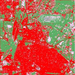
 NN
NN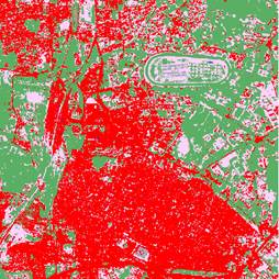
 RF
RF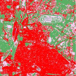
 SMAP
SMAP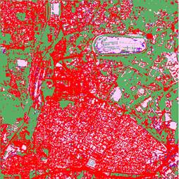 SVM (Polynomial)
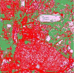 SVM (RBF)