DATA AND METHODS

• Study area: The study has been carried out for a rapidly urbanizing region in India. Greater Bangalore is  the  administrative,  cultural,  commercial,  industrial,  and knowledge capital of the state of Karnataka, India with an area of 741 sq. km. and lies between 12°39’00’’  to  13°13’00’’ N  and  77°22’00’’  to  77°52’00’’ E (Fig. 4.1). Bangalore city administrative jurisdiction was redefined in the year 2006 by merging the existing area of Bangalore city spatial limits with 8 neighboring Urban Local Bodies (ULBs) and 111 Villages of Bangalore Urban District. Bangalore has grown spatially more than  ten times  since  1949  (~69  square  kilometers to 741 square kilometers)  and  is  the  fifth  largest  metropolis  in  India currently with a population of about 8.5 million [92, 93]. Bangalore city population has increased enormously from 65,37,124 (in 2001) to 95,88,910 (in 2011), accounting for 46.68 % growth in a decade. Population density has increased from 10,732 (in 2001) to 13392 (in 2011) persons per sq. km [94, 95]. The per capita GDP of Bangalore is about $2066, which is considerably low with limited expansion to balance both environmental and economic needs.

Table 1.1 and Fig. 4.2 gives an insight to the temporal land use changes during 1973 to 2013 (based on the analyses of spatial data acquired remotely at regular time intervals since early seventies through space borne sensors). The built-up area has increased from 7.97% (in 1973) to 58.33 % in 2012 and 73.72% in 2013. The sudden increment in urbanization during post 1990’s was due to the globalization and consequent industrialization (in Peenya, Rajajinagar, Koramangala). Post 2000, Government’s push to software sectors led to the large scale land use changes with urbanization at White field, Electronic city, Domlur, Hebbal, due to private players and development of Special Economic Zones (SEZ). Bangalore, once branded as the Garden city due to dense vegetation cover, which has declined from 68.27% (1973) to less than 15% (2013). The temporal analyses of spatial data also reveals of 925% increase in buit-up (building, roads, etc.) with the decline of 78% vegetation and 79% of area covered with water bodies [96, 97] during 1970 to 2013.  Developments in various fronts with the consequent increasing demand for housing have urbanized these regions evident from the drastic increase in the urban density during the last two decades. Bangalore grew intensely in the north-west (NW) and south west (SW) regions in 1992 due to the policy of industrialization consequent to the globalization [97]. The industrial layouts came up in NW and housing colonies in SW and urban sprawl was noticed in others parts of the Bangalore. This phenomenon intensified due to impetus to IT (Information Technology) and BT (Biotechnology) sectors in south-east (SE) and north-east (NE) during post 2000. Subsequent to this, relaxation of FAR (Floor area ratio) in mid-2005, lead to the spurt in high raise buildings in residential and commercial sectors, paved way for large scale conversion of land leading to intense urbanisation in many localities. This also led to the compact growth at central core areas of Bangalore and dispersed growth at outskirts. These sprawl regions are devoid of basic amenities and infrastructure. The analysis showed that Bangalore grew radially from 1973 to 2014 indicating that the urbanisation has intensified from the city center and reached the periphery of Greater Bangalore.

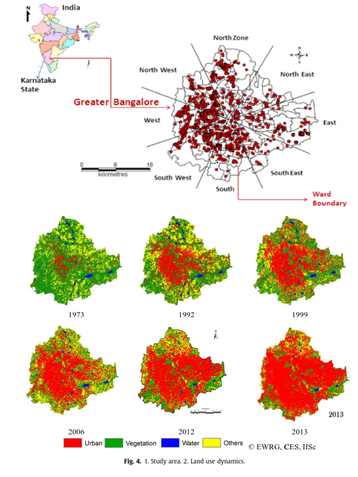
Table 1: Temporal Land use dynamics in Bangalore

Similar trends of urbanisation are noticed in other major metropolitans - Kolkata, Mumbai, Chennai and Delhi, which recorded an urban growth of 425% [98], 467% [99], 650% [100] and 850% [101]. Mumbai is the commercial capital of India has a GDP of 209 Billion USD, followed by Delhi (167 Billion USD), Kolkata (150 Billion USD). Bangalore (85 Billion USD) and Chennai (66 Billion USD).  Assessment of GHG footprint (Aggregation of Carbon dioxide equivalent emissions of GHG’s) of Delhi, Greater Mumbai, Kolkata, Chennai, Greater Bangalore, Hyderabad and Ahmedabad are found to be 38633.2 Gg, 22783.08 Gg, 14812.10 Gg, 22090.55 Gg, 19796.5 Gg, 13734.59 Gg and 9124.45 Gg CO2 eq respectively. Chennai emits 4.79 tonnes of CO2 equivalent emissions per capita, the highest among all the cities followed by Kolkata which emits 3.29 tonnes of CO2 equivalent emissions per capita. Also Chennai emits the highest CO2 equivalent emissions per GDP (2.55 tonnes CO2 eq/lakh Rs.) followed by Greater Bangalore which emits 2.18 tonnes CO2 eq/lakh Rs. [102].

• Data collection: Assessment of the spatial patterns in GHG emissions due to domestic energy consumption involved i) primary survey of sample household through the pretested and validated structured questionnaire and ii) compilation of ward wise electricity consumption data from the government agencies. Bangalore with a spatial extent of 741 sq.km has 198 administrative wards. Wards were prioritized for sampling based on type, economic activities and social aspects. The survey was carried out during 2011-12 in select households chosen based on stratified (economic status) random selection and validation of sampled data was done during 2012-14. Survey covered 1967 households representing heterogeneous population belonging to different income, education, and social aspects. Fig. 4.1 gives the spatial distribution of sampled household (marked as red dots in the study area - Bangalore). The questionnaire was designed to explore key drivers which affect household energy consumption, physical characteristics of dwelling (residential status, type of building, year of house unit built), attitude towards surrounding environment and other parameter includes household size, annual income, age, energy consumption behavior of households. Energy consumption in a household is an outcome of various household behavior such as type of water heating systems (solar, electricity, LPG, etc.), type of fuel used for cooking (electricity, LPG, fuel wood), details of electrical gadgets (lighting, electric fan, refrigerator, washing machine, water treatment units, computers, television, computers, laptop, etc.). Secondary data of ward wise annual electricity consumption for the period 2001 to 2013 was collected from the BESCOM (Bangalore Electricity Supply Company).  

• Method of analysis: Spatial patterns in energy consumption and GHG emission is assessed considering various growth poles based on the extent of urbanization. The study area was divided into 8 zones (/regions) based on directions –North, Northeast (NE), East (E), Southeast (SE), South, Southwest (SW), West (W), Northwest (NW), respectively (Fig. 4.1) based on the Central pixel (Central Business district, CBD). The electricity and LPG consumptions were computed for each zones based on the compiled data through sample surveys in each zones.

Emission due to electricity use in the domestic sector is quantified using Eq. (1) considering quantity of electricity consumption and emission factor. The emission factors and net calorific values (NCV) for different sectors are listed in Table 2.
C= βE                                          … (1)
Where, C is carbon dioxide emission; β is emission factor (Table 2) and E is consumption of electricity.

Table 2: Emission factors and net calorific values (NCV)

Liquefied Petroleum Gas (LPG) is the principal fuel used for cooking in the residential sector.   Emission due to LPG consumption is computed using Eq. (2).

E = Fuel * NCV * EFGHG                          … (2)

Where E is the emission; Fuel quantity consumed; NCV is net calorific value; EFGHG is the emission factor of LPG (given in Table 2)