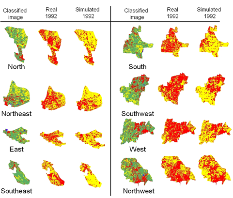
Figure 6. Classified images of 1973, real image and simulated image of 1992. Red colour indicates urban areas, yellow represents other classes (vegetation, water or open land) in real and simulated images.

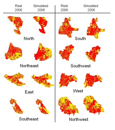
Figure 7. Real image and simulated image of 2006. Red colour indicates urban areas, yellow represents other classes (vegetation, water or open land).

Prediction accuracy for each direction was used as a basis for rule calibration. If a set of rules for a particular direction produced underestimated results, then it means the growth rate was small and hence the rules were modified to increase the urban growth. For overestimation, the rules were modified to reduce the urban growth. The transition rules for a direction were repeatedly calibrated till the convergence criterion was met. The classified image provides the reference for calibration process. In table 2, the Fitness %, Total Error (∆E %) and f values for the year 1992 indicates poor match of the simulated image with the real image (classified image), which is an indication of underestimation of urban pixels in various directions. However, the results for the 2006 simulated image (table 2) indicate very good spatial prediction accuracy. The spatial variability between various directions as compared to the real image is small. This indicates the effect of spatial calibration in matching each direction with its realistic urban growth pattern through calibrating its rules. It also helped in capturing finer details, while calibrating the model over smaller spatial units to reduce modelling uncertainty. Visually, calibration on a directional basis succeeds in preserving the urban pattern over space and over time. Rule values’ results at the end of the calibration process indicate similarity between growth in various directions such as in the east, west and northwest.

In reality, these wards have almost the same growth rate and pattern because of similar infrastructure, facilities, and more open area for outer growth and urban sprawl. Most of these similar wards have ring roads or highways passing through them that allow linear urban growth happening along them. The average fitness value for the 1992 image was ~ 60% and the total error was 29.09 with an approximate match of 71%. It is to be noted that for a highly accurate prediction, the total modelled urban count and ground truth urban count will be equal and therefore the fitness value (F) will be 1 or 100%. The total error ∆E is the error of omission and commission. More the value of ∆E, more is the percentage of error count. There seems to be some mismatch between the actual and simulated urban pixel patterns in 1992 as this pattern was not captured accurately by the change in population density contours and curve fits in various wards and different directions. Simulation and prediction urban modelling results, as shown in table 2 for the year 2006, show that the fitness results for prediction was close, in terms of urban count, (values close to 100%) between the modelled and real data with average fitness of 101.60 (which is a slight overestimate) and the average total error of 31.68% was achieved. This indicates an approximate match level of 69% on a pixel by pixel basis between modelling and reality. Therefore, higher the value of f in equation 8, higher is the modelling error. For the 2006 simulated image, the average f is 33.33, showing a more realistic result compared to the actual urban growth pattern. This is a high accuracy level compared to the results shown in literatures for the urban land spatial fit area that was only 28.15 to 44.6% (Yang and Lo, 2003). The close urban pattern match is also clear in figure 7 where the simulated images have urban distribution similar to those shown in their corresponding real images. This indicates the ability of CA based modelling and calibration in spatial and temporal domain and also proves their effectiveness in understanding human-environment interactions to a great extent. Based on the objective of this study, cell space, cell states, neighbourhood, growth constraint, and calibration followed by validation were carried out using simple CA models for complex dynamic urban systems. The state of any cell depends upon some function which reacts to what is already in that cell as well as some function which relates the cell to what is happening in its immediate neighbourhood, that is the diffusion component (Batty, 1999). The most attractive property of CA models for simulating urban systems is that local action in such models can give rise to global forms which evolve or emerge spontaneously with no hidden hand directing the evolution of the macrostructure (Batty et al., 1999). They can help in interpreting, modelling, predicting and understanding the dynamics of natural resources.

Comparison of CA models with other urban process models highlight certain merits, but there are drawbacks such as (i) Relaxation of the original scheme of CA may lead to the loss of fundamental characteristics of simplicity and locality, or loss in the model in which the CA component is no longer the core. (ii) CA models are not suited to define general urban CA, but are rather a methodology to define specific models for each situation. (iii) CA generally produce descriptive models that tell us what is happening but it does not tell us why? (iv) Data requirements depend upon the factor considered in the model and so, they are usually in opposition to flexibility (Sante et al., 2010). Further research in this direction is required for focussing on the drawbacks such as transition rules considering road accessibility, distance to multiple urban centres in the city, slope, accessibility to railway, site suitability for development, population density, etc.