 |
Cellular Automata Calibration Model to Capture Urban Growth
|
 |
Uttam Kumar1,4,5, Chiranjit Mukhopadhyay4, T.V. Ramachandra1,2,3*
1Energy & Wetlends Research Group, Center for Ecological Sciences [CES], Indian Institute of Science,
2Center for Sustainable Technologies (astra), Indian Institute of Science,
3Centre for infrastructure, Sustainable Transportation and Urban Planning [CiSTUP]
4Department of Management Studies
5International Institute of Information Technology, Bangalore-560100, India
*Corresponding author:
Energy & Wetlands Research Group,
Centre for Ecological Sciences
Indian Institute of Science,
Bangalore – 560 012, INDIA, E-mail: cestvr@ces.iisc.ac.in, energy@ces.iisc.ac.in.
Area of Study, Data and methodology
This section describes the study area and input data processing scheme. The study area considered is Bangalore city, which is the principal administrative, cultural, commercial, industrial, and knowledge capital of the Karnataka state in India. The administrative jurisdiction was widened in 2006 by merging the existing area of Bangalore city spatial limits with eight neighbouring Urban Local Bodies and 111 Villages of Bangalore Urban District to form Greater Bangalore. Bangalore has spatially grown to more than ten times from 69 to 741 square kilometres from the year 1949 to the year 2006. Now, Bangalore is the third largest metropolis in India currently with a population of about 9.6 million (Census of India, 2011; Ramachandra et al., 2008). Bangalore city is composed of 100 wards. Since, urbanisation and urban sprawl are more of a local phenomenon and site specific, local urban sprawl tends to increase in a certain direction along ring roads, highways, or around service facilities in another direction, which later become the urban centre hub. The greater the distance from the city centre, the less is the development (Cheng and Masser, 2004;Li and Yeh, 2002; Yeh and Li, 2001). Therefore, a better way to understand the spatio-temporal pattern of a city is to study the urban landscape in different directions from the central business district. For this reason, in the current study, the city was divided into 8 zones [North (N), Northeast (NE), East (E), Southeast (SE), South (S), Southwest (SW), West (W), and Northwest (NW)] with their origin from the ‘city centre’ as shown in figure 1. Visualisation of the sprawl process is crucial in urban planning for providing basic amenities in different geographical locations.
The two types of input data were:
(i) classified RS data of 1973, 1992 and 2006.
(ii) population density maps for the year 1973 and 1992.
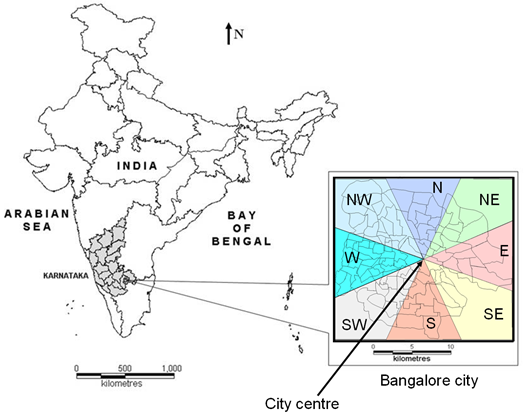
Figure 1. Study area: Bangalore city, Greater Bangalore, India.
Landsat Multispectral Scanner (MSS) of 1973 (in Blue (B), Green (G), Red (R) and Near Infrared (IR) bands of 79 m spatial resolution), Landsat Thematic Mapper (TM) of 1992 (B, G, R, Near IR, Mid IR-1 and Mid IR-2 bands of 30 m spatial resolution), and IRS Linear Imaging Self Scanner (LISS) -III of 2006 (in G, R and NIR bands of 23.5 m spatial resolution) were used for the generation of land use maps. The data are stored in 8-bit format, i.e. each pixel can take any value from 0 to 255 (28= 256 values) which represents the reflectance by that pixel corresponding to the same geographical location on the ground. The 1973 image was of the dimension 429 rows x 445 columns, whereas 1992 image was of 1130 rows x 1170 columns and 2006 image was of 1445 rows x 1496 columns. The differences in the size of the images are due to variations in the spatial resolution of the pixels (79 m, 30 m, and 23.5 m respectively). These data were rectified and registered for systematic errors with known ground control points that were identifiable both in the image as well as in the Survey of India (SOI) Topographical sheets of 1:50000 scale and projected to Polyconic system with Geographic Latitude-Longitude coordinate system and Evrst56 as the datum. All data were resampled to have 23.5 m spatial resolution having 1445 rows x 1496 columns to fit each other spatially. Six classes of interest were identified from the false colour composite images: residential areas, commercial areas, roads, vegetation, water, and open land.
Supervised classification of the image was performed using Maximum Likelihood classifier (MLC). MLC has become popular and widespread in RS because of its robustness (Conese and Maselli, 1992; Ediriwickrema and Khorram, 1997; Strahler, 1980;Zheng et al., 2005). MLC assumes that each class in each band can be described by a normal distribution (Bayarsaikhan et al., 2009). For each land use class (residential areas, commercial areas, roads, vegetation, water, and open land), training samples / polygons were collected using hand held GPS from across the city, representing approximately 10% of the study area. With these 10% known pixel labels from training data, the aim was to assign labels to all the remaining pixels in the image (RS data of Bangalore city). The objective was to classify a pixel with M x 1 grey scale values, corresponding to M spectral bands, into one of the N spatial classes.
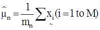
At the outset, let the spectral classes in the data be represented by ωn, n=1,…, N, where N is the total number of classes, and . Let denote the (m x 1) grey-scale values across the M spectral bands of mn sampled pixels (observations or training samples which are independent and identically distributed (i.i.d.) random variables), belonging to the nth spatial class, then
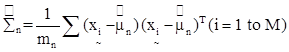
Bayes’ decision theory forms the basis of statistical pattern recognition based on the assumption that the decision problem can be specified in probabilistic terms (Wölfel and Ekenel, 2005). The MLC assuming the distribution of data points to be Gaussian, quantitatively evaluates both the variance and covariance of the category’s spectral response pattern (Lillesand and Kiefer, 2002) which is described by the mean vector and the covariance matrix. The statistical probability of a given pixel value being a member of a particular class is computed and the pixel is assigned to the most likely class (highest probability value).
p(ωn|x) gives the probability that the pixel with observed column vector of DNs (digital numbers) x, belongs to class ωn. It describes the pixel as a point in multispectral (MS) space (M-dimensional space, where M is the number of spectral bands). The maximum likelihood (ML) parameters are estimated from representative i.i.d. samples. Classification is performed according to
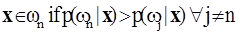 ________________________ ( 1 ) ________________________ ( 1 )
i.e., the pixel vector x belongs to class ωn if p(ωn|x) is largest. The ML decision rule is based on a normalised estimate of the probability density function (p.d.f.) of each class. MLC uses Bayes decision theory where the discriminant function, gln(x) for ωn is expressed as
 __________________________( 2 ) __________________________( 2 )
Where p(ωn) is the prior probability of ωn, p(x|ωn) is the p.d.f. (assumed to have a Gaussian distribution for each class ωn) for pixel vector x conditioned on ωn (Zheng et al., 2005). Pixel vector x is assigned to the class for which gln(x) is greatest. In an operational context, the logarithm form of (2) is used, and after the constants are eliminated, the discriminant function for ωn is stated as
 ______________________( 3 ) ______________________( 3 )
where is the variance-covariance matrix of , is the mean vector of . Equation (3) is a special case of the general linear discriminant function in multivariate statistics (Johnson and Wichern, 2005) and used in this current form in the RS digital image processing community. A pixel is assigned to the class with the lowest in equation (3) (Duda et al., 2000; Richards and Jia, 2006; Zheng et al., 2005).
Residential and commercial areas, and roads were grouped into a single class called ‘urban’. Final classified images thus had four land use classes – urban, vegetation, water and open land (others). The classified images of 1973, 1992 and 2006 had overall accuracies of 72%, 75%, and 73% respectively. Classification was done using the open source programs (i.gensig, i.class and i.maxlik) of Geographic Resources Analysis Support System (http://wgbis.ces.iisc.ac.in/grass) and is displayed in figure 2. The classified images were also verified with field visits and Google Earth images. The class statistics is given in table 1.
Class à
Year â |
Urban |
Vegetation |
Water Bodies |
Open land |
1973 |
Ha |
5448 |
46639 |
2324 |
13903 |
% |
7.97 |
68.27 |
3.40 |
20.35 |
1992 |
Ha |
18650 |
31579 |
1790 |
16303 |
% |
27.30 |
46.22 |
2.60 |
23.86 |
2006 |
Ha |
29535 |
19696 |
1073 |
18017 |
% |
43.23 |
28.83 |
1.57 |
26.37 |
Table 1.Greater Bangalore land use statistics
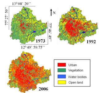
Figure 2. Greater Bangalore in 1973, 1992 and 2006.
Population density is a second input that is required for the CA modelling. Population map of Bangalore city was prepared from the Census of India data of 10 years interval (1971, 1981, 1991, 2001). The Indian Census by the Directorate of the census operation, Government of India (http://censusindia.gov.in) is the most credible source of information on Demography (Population characteristics), Economic Activity, Literacy and Education, Housing & Household Amenities, Urbanisation and many other socio-cultural and demographic data since 1872. Population densities for all 100 wards were computed by dividing their populations by their respective ward areas. Figure 3 shows the ward map (left) in each direction and the population density for each ward (a basic administrative unit) (right) in 1971, 1991 and 2001.
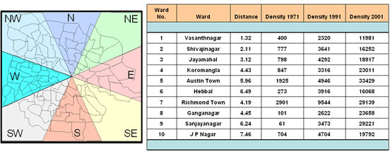
Figure 3. Ward map in each direction and their population densities. Distances are expressed in kilometres and population densities are expressed in persons/sq. km.
Population densities for 1973, 1992 and 2006 were extrapolated from the population densities of 1971, 1991 and 2001 to correspond with RS data. First, the centroid for each ward was calculated. Then, the Euclidean distance from each ward centroid to the city center (see figure 1) was computed. This process was repeated for all wards to prepare a table of population densities versus distance. Population densities for wards within specified distance from the city center were averaged to reduce the variability in data. For example, an average population density for all wards within 0-1 km was calculated, then another average density was calculated for wards within 1-2, 2-3, 3-4 km and so on. Curves were fitted representing population density as a function of distance from the city centre as shown in figure 4. The unknown model parameters in the curve fitted equations were calculated for the years 1991 and 2001. These models were used to calculate the population density for each pixel in the imagery based on its distance from the city center for the years 1991 and 2001. The changes in model parameters over the 10 years (from 1991 to 2001) were used to calculate the yearly rate of change. The updated parameters that changed year by year were used to calculate the population density grids for the years 1973 and 1992 matching the same size of the input imagery (classified maps - 1445 rows and 1496 columns). These grids were used as input to the CA model.
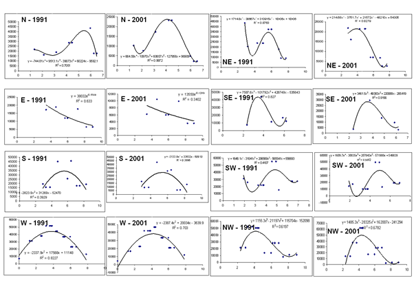
Figure 4. Direction wise population density for the year 1991 and 2001.
CELLULAR AUTOMATA (CA) GROWTH MODELLING
This section discusses the design of CA urban growth modelling in detail. The CA algorithm consists of defining the transition rules that control the urban growth, calibrating these rules, and then evaluating the results for prediction purpose.
TRANSITION RULES
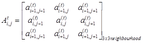
Transition rules translate the effect of input data in simulating the urbanisation process. The CA algorithm design starts by defining the transition rules that drive the urban growth over time. They depend on the current status of land usage, population density and are subject to certain growth constraints. The transition rules are defined for the 3 x 3 neighbourhood of a pixel. The rules identify the neighbourhood needed for the tested cell to urbanise.
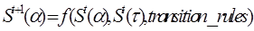
The growth constraints reflect urbanisation strategies adopted in the study area for certain land uses such as conservation of the water bodies (lakes). Urban growth in the vicinity of such sites is constrained by imposing rules that discourage urbanisation into water bodies. The future state of a pixel at time (t+1) from the current time (t) depends on three factors: (i) current state of the pixel, (ii) current states of the neighbourhood pixels, and (iii) transition rules that drive the urban growth over time, which may be represented by
 ____________________( 4 ) ____________________( 4 )
where
 =Future state of pixel α at time epoch t+1 =Future state of pixel α at time epoch t+1
 = Current state of pixel α at time epoch t = Current state of pixel α at time epoch t
 = State of pixel , which is a neighbourhood pixel of pixel α. = State of pixel , which is a neighbourhood pixel of pixel α.
Transition rules (f) were designed to identify the required neighborhood urban level for a test pixel to urbanise. The following rules were adopted from AlKheder et al., (2007): If the pixel being transformed is either water, road, residential or commercial, then perform no change, otherwise if the pixel belongs to vegetation or open land, then its state will be altered to urban, provided the population density is ≥ threshold (P) and the number of surrounding urban pixelsare ≥ threshold (R). R is an integer ranging from 0 to 8 (3x3 neighborhood) and P is a real number ranging from 0 to 1 (0.1 increment; population density values were normalized from 0 to 1 for each direction in order to have effective CA rules calibration).
CALIBRATION
The calibration of urban CA model is done to determine optimal weights or parameters of the transition rules such as P or R mentioned above (Dietzel and Clarke, 2006; Li and Yeh, 2001; Li et al., 2007; Stevens et al., 2007; Wu, 2002). Calibration is an integral part of the CA model design and development process as it is in this step that one attempts to ensure that the model provides reasonable predictions about current and future scenarios (Li and Yeh, 2001, 2002; Waddell, 2005). It aims to define the optimal set of CA rules such that the agreement between simulated results and ground truth images are as best as possible.
The relaxations allowed in CA helped in simulating more realistic urban growth that led to the emergence of a large variety of rules. To achieve this, two calibration schemes were used, namely spatial and temporal calibrations. In spatial calibration, the CA transition rules at a given time t were modified spatially over the 2D grid space by tuning the values of each rule set on a directional basis to match the urban dynamics for each ward with its site specific features, allowing the model to take the variability in the spatial urban growth pattern into account for realistic modelling. If the transition rules in a given direction resulted in higher growth levels (overestimated), they were modified to reduce the urban growth in that direction. In case of underestimation, the rule values of the direction under consideration were tuned to increase the amount of urban growth to match the real one. Therefore, spatial calibration is meant to find the best set of rule values that best fits a given direction according to its geographical location. This is similar to the SLEUTH model (Silvaand Clarke, 2002), where the parameters can be set best that simulates the application data by narrowing both the spatial scale and the range of parameters in the calibration sequences. These parameters are then used to determine the parameter values that optimally allow the model to run into the future, i.e. to predict.
The oldest classified Landsat MSS image (of 1973) of Bangalore city (figure 5) obtained by subsetting Greater Bangalore image (figure 2) was used as input to the CA model over which the transition rules were applied to model the urban growth starting from this time epoch. Dividing the study area on a direction (or zones such as N, NE, E, SE, S, SW, W, and NW as explained in section 3) and further on a ward basis took into consideration the effect of site specific features spatially. The same CA transition rules were defined for each direction, however, with different rule values. CA transition rules (f) of the developed model were physically built over the input imagery and the rules used a 3 x 3 neighbourhood - in equation 5 to identify the test pixel’s future state, in equation 6.
 ______________( 5 ) ______________( 5 )
 ______________( 6 ) ______________( 6 )
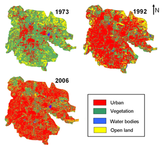
Figure 5. Bangalore city in 1973, 1992 and 2006 used in the CA model for simulation (subset of Greater Bangalore classified image).
The calibration (i.e., identifying best (R,P) parameter values) of such rules was performed spatially on a ward level, Tw (where w represents individual wards) to fit the local urban dynamic features and over time to consider the temporal urban changes in each direction, Tt (where t represents time in years) in equation 7.
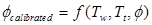 __________( 7 ) __________( 7 )
f in the calibration formula represents the criteria selected to find the best rule set for certain ward spatial location Tw at given time epoch Tt. This criterion in the model represents the total modelling errors/mismatch between modeled output and reality that need to be minimised or best matched. f in equation 8 was defined as a function of fitness F in equation 9 and total errors ∆E in equation 10. Fitness and total errors measure the compatibility in terms of urban count and pattern within each ward with respect to reality, respectively (Al-Kheder, et al., 2007)
. 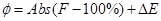 _______________( 8 ) _______________( 8 )
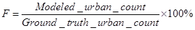 _______________( 9 ) _______________( 9 )
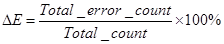
________________(10)
Once the CA transition rules were identified and initialised for each direction, the model was run from 1973 till 1992. The 1992 image represents the first ground truth being used for calibration. For each ward, the modelling accuracy is calculated as a ratio between the simulated and real urban growth data. Over/underestimation is introduced to represent how comparable the simulated result is to the real one. This indicates how transition rules defined on a directional basis succeed in modelling the real urban growth given the predefined conditions. Calibration is meant to find the best set of rule values specific to each direction for realistic urban growth modelling.
Citation :U. Kumar, C. Mukhopadhyay, T. V. Ramachandra, 2014. Cellular Automata Calibration Model to Capture Urban Growth. Boletín Geológico y Minero, 125 (3): 285-299 [Best Paper Award, Boletín Geológico y Minero].
|
|
|