Materials and Methods

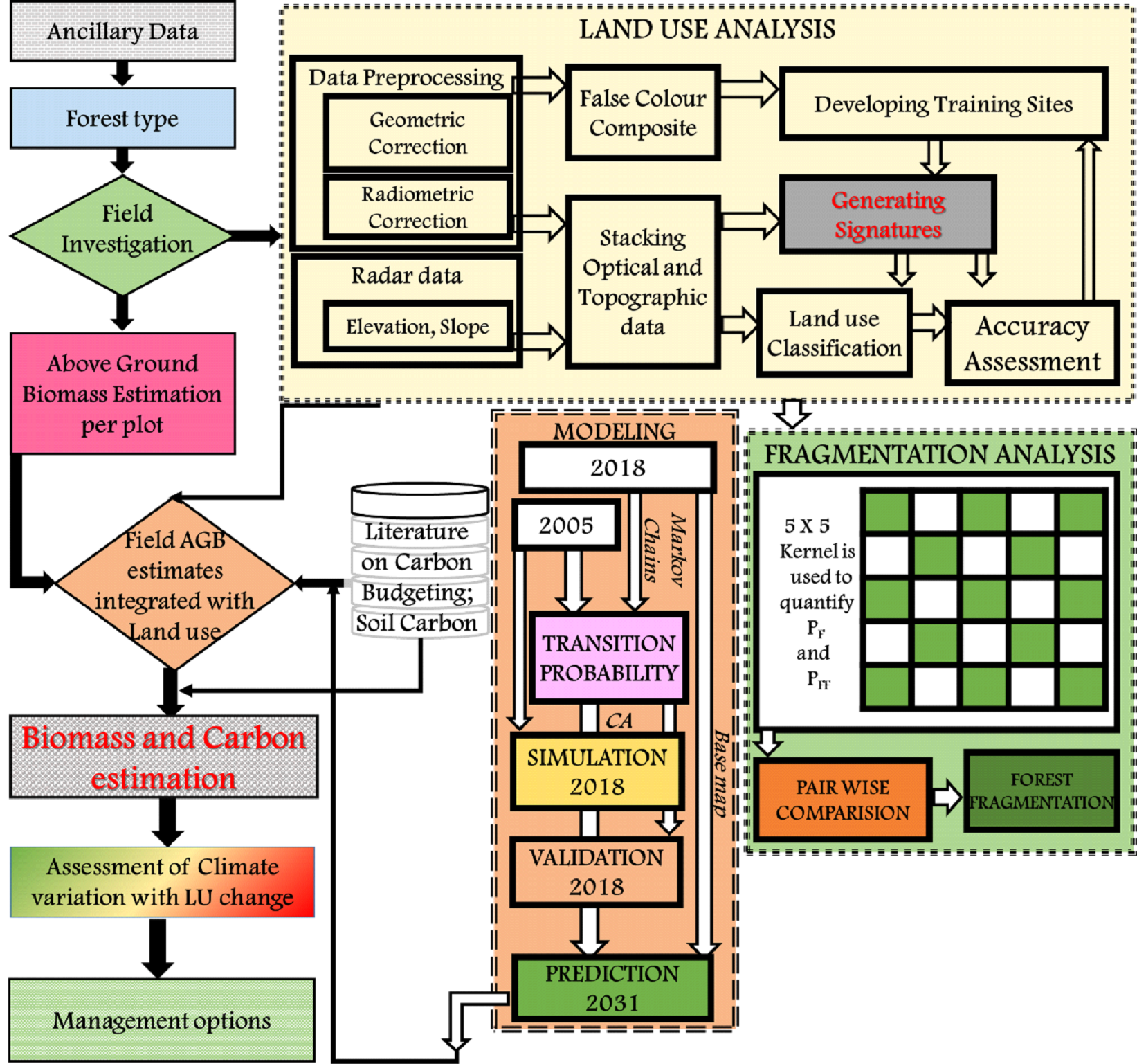
The approach followed to quantify carbon sequestration potential of WG and climate variation are explained in Fig. 2, which included (i) the spatial analyses of LU dynamics and modeling, (ii) carbon sequestration potential of forests ecosystems in WG, (iii) assessment of climate variability with LU dynamics.

Quantification and Modeling of LU changes

The LU analysis is performed by using the Landsat 8 Operational Land Imager (OLI-30 m resolution) 2018 data integrated with field estimations and decadal land use (1985, 1995, 2005-100 m resolution) available from International Geosphere-Biosphere Programme (IGBP). The collateral data included the vegetation maps developed by French institute Puducherry, topographic maps (the Survey of India) and virtual earth data (Google Earth, Bhuvan). GPS and AGPS based field surveys were done in order to supplement LU analysis and geometric correction. The process of classification involves the (i) creation of false color composite (FCC) using 3 bands of LANDSAT data, which helped in identifying the heterogeneous regions and the selection of training sites, (ii) collection of attribute data from the field for the training polygons and virtual data (Google Earth, Bhuvan), (iii) LU classification information derivation from RS data through Gaussian Maximum likelihood algorithm using training data and (iv) accuracy assessment through computation of error metrix (confusion metrix) and kappa statistics. The Gaussian maximum likelihood classifier (GMLC) is proved to be an efficient supervised classification technique for deriving 8 different LU categories from RS data (Vinay et al. 2013; Bharath et al. 2014; Ramachandra et al. 2016; Ramachandra and Bharath 2018) using free and open source GRASS GIS (Geographical Analysis Support System - http://wgbis.ces.iisc.ernet.in/grass/). The training data (60%) collected has been used for classification, while the balance used for accuracy assessment and validation (Lillesand et al. 2014).

Fig. 2 Method used for the analysis

Assessment of climate variability and trend with LU changes

The forest fragmentation has been analysed using two prime indicators such as P_f, P_ff (cardinal direction) as shown in equations 1 and 2 (Riitters et al. 2002; Ramachandra et al. 2016). P_f and P_ff were computed as per equations 1 and 2, through a moving window of 5×5 pixels in order to maintain a fair representation of the proportion as given that the results of the model are scale dependent and threshold dependent (Riitters et al. 2000; 2002; Kuèas et al. 2011). Water bodies or river courses are considered non-fragmenting features, and constitute natural corridors in a forested landscape, while anthropogenic landscape elements (such as buildings, roads, agricultural field and barren land) are drivers of forest fragmentation.

P_f = Proportion of number of forest pixels/Total number of non - water pixels in window (1)
P_ff = Proportion of number of forest pixel pairs/Total number of adjacent pairs of at least one forest pixel (2)

The constrained Cellular Automata and Markov chain (CA-Markov) has been used for the simulation of likely LU (2031). The CA-Markov modeling technique has been widely used and efficient technique for LU simulation across the globe due to its simplicity and predictive power (Fu et al. 2018). CA-Markov uses the spatial arrangement, states, neighborhood, rules of transition, temporal scale of cells for enhanced simulation (Arsanjani et al. 2013). Water bodies or river courses and protected areas are considered as constraints of LU change. The transition probability and area metrics were generated and used for the simulation as outlined in Bharath et al. (2014).

Carbon sequestration potential of forests and its future status

The carbon sequestration potential of forest ecosystems was assessed based on (i) published literature based on the standard biomass experiments and (ii) field based measurements collected across the forests of WG of Karnataka using transect based quadrat sampling techniques (Fig. 3). The field estimations were done across the varied forest types covering around 300 transects in Uttara Kannada, Shimoga, Chikmagalur, Kodagu, Dakshina Kannada and Udupi districts. The WG is divided into 5’ × 5’ grids (2300) for biomass and carbon estimation. The biomass was estimated using GBH (girth at breast height) for the trees >30 cm. The transect data and standard literature data used for the quantification.

The Western Ghats consists of three diverse agro climatic zones namely (i) coastal, (ii) Sahyadri interior and (iii) Plains. Probable relationship between basal area (BA), and forest cover and extent of interior forest, given in equation 3 is based on the field data (standing biomass) coupled with land use data (land use – forests and interior forest / contiguous forests from the fragmentation analyses).

Fig. 3 Transect cum quadrat method

The multivariate statistical analysis was done for estimating the relationship between a dependent (standing biomass) and independent variables (basal area, forest cover, percentage of interior forests-computed from land use analysis). The standing biomass and carbon stock in each grid of Western Ghats region were quantified as per eq. 3,

standing biomass = F {basal area f ; interior forest;forest coverg }(3)

Statistically significant equations based on the basal area with land use and interior forest were obtained and given in equations 4, 5, and 6 respectively for coastal, Sahyadri and plains. Validation of basal area based on equation 2-4 was done with the known basal area (colleted through field sampling) in the respective grids. Later, basal area (Table 2) for all grids in the coast, Sahyadri interior and plains were computed considering forest land use and interior forests (in the respective grids) using equations 4, 5 and 6.

Coastal regions,

BA = {30.1 + (0.0414 * (forest land use) +0.053 * (interior forest) ; n = 50; SE = 6.2 (4)
Sahyadri interior regions:
BA = {39.1 + (-0.099 * (forest land use) + 0.091 * (interior forest) ; n = 55; SE = 6.3 (5)
Plain regions:
BA = {34.8 + (-0.186 * (forest land use) + 0.12 * (interior forest) ; n = 11; SE = 5.5 (6)

Where n is a number of transects and SE refers to standard error. Comparisons of predicted (as per equations 2,3 and 4 for different agro-climatic regions) and quantified basal area from the field showed a reasonable agreement with the co-efficient of determination (R) of 0.878 and standard error of 11.73. Parameters such as annual increment of biomass (standing biomass) and carbon were evaluated based on field measurement and the review of literatures based on forest types as listed in Table 1. Carbon storage in forests is estimated by taking 50% of the biomass as carbon. The carbon is stored in the soil as soil organic matter (SOM) in both organic and inorganic forms. Soil carbon is calculated based on the field estimations in top 30 cm soil for different forests and extrapolated for all grids as per Table 2. Sequestered carbon, annual increment of carbon has been computed considering various land use types as per Table 3.

Assessment of Climate Variability and Trend with Land-Use Changes
Daily rainfall and temperature data (of 0.50º resolution) for the period 1901 and 2017 were collated from Princeton University Database (Princeton data—THRG 2019), NCAR climate data guide (NCAR 2019), Indian Meteorological Department (IMD 2018) and Local climate data (Karnataka State Natural Resource Disaster Monitoring Centre (KSNDMC 2018)). Princeton data and NCAR data were validated at latitude levels by comparison with the surface measurements of IMD and local climate data. The mean and variance were computed and compared, which illustrates the global data are comparable to surface measurements (with deviation £ 4.3%) These climatic data at latitude level were further analyzed for variability and trend. Climate (rainfall and temperature) data were compared with land-use changes to understand the role of land-use in the regional climate variability.

Table 1. Above ground Biomass for various forest types

Sno	Forest Type	Standing Biomass (t/ha)
1	Dense Evergreen to Semi evergreen	485.67 to 833.22
2	Low evergreen	226.55
3	Dense Deciduous	258.12
4	Degraded Deciduous	129.92
5	Savanna Woodlands	74.25 to 90
6	Thorn degraded	40
7	Littoral and swamp	213.8