
In order to understand the spatial pattern of urbanization, eleven landscape level metrics were computed zonewise for each circle. These metrics are discussed below:
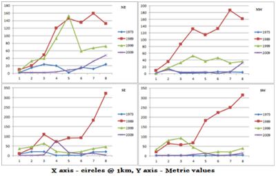
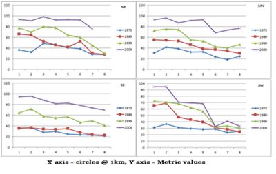
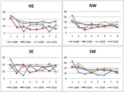
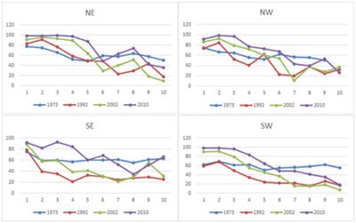
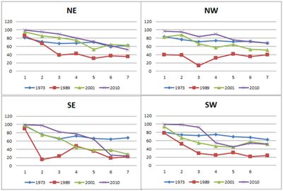
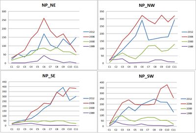
7.1 Mysore: Number of Urban Patch (Np) is a landscape metric indicates the level of fragmentation and ranges from 0 (fragment) to 100 (clumpiness). Figure 10a illustrates that the city is becoming clumped patch at the center, while outskirts are relatively fragmented. Clumped patches are more prominent in NE and NW directions and patches is agglomerating to a single urban patch. Largest patch index (Fig 10b) highlights that the city’s landscape is fragmented in all direction (in 1973) due to heterogeneous landscapes, transformed a homogeneous single patch in 2009.The patch sizes given in figure 8c highlights that there were small urban patches in all directions (till 1999) and the increase in the LPI values implies increased urban patches during 2009 in the NE and SW. Higher values at the center indicates the aggregation at the center and in the verge of forming a single urban patch largest patches were found in NE and SW direction (2009).
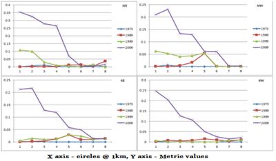
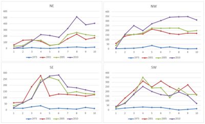
The patch density (Fig 10c) is calculated on a raster map, using a 4 neighbour algorithm. Patch density increases with a greater number of patches within a reference area. Patch density was higher in 1973 as the number of patches is higher in all directions and gradients due to presence of diverse land use, which remarkably increased post 1989(NW) and subsequently reduced in 1999, indicating the sprawl in the region in in early 90’s and started to clump during 2009, which was even confirmed by number of patches.
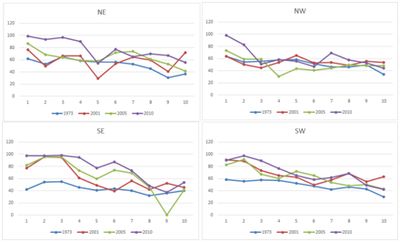
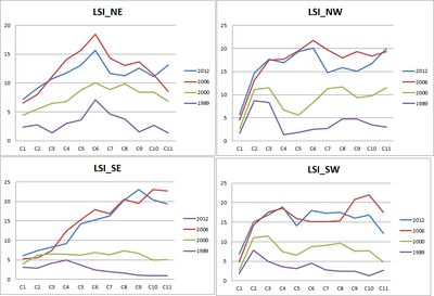
Landscape Shape Index (LSI): LSI equals to 1 when the landscape consists of a single square or maximally compact (i.e., almost square) patch of the corresponding type and LSI increases without limit as the patch type becomes more disaggregated. Results (Fig 10d) indicate that there were low LSI values in 1973 as there was minimal urban areas which were aggregated at the centre. Since 1990’s the city has been experiencing dispersed growth in all direction and circles, towards 2009 it shows a aggregating trend as the value reaches 1.
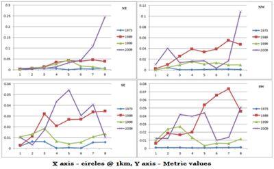
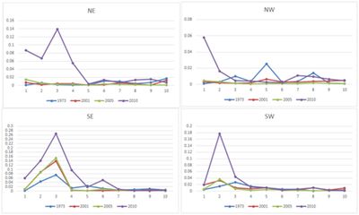
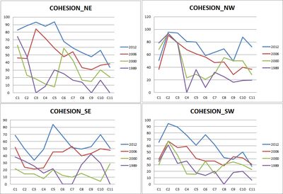
Patch cohesion index measures the physical connectedness of the corresponding patch type. This is sensitive to the aggregation of the focal class below the percolation threshold. Patch cohesion increases as the patch type becomes more clumped or aggregated in its distribution; hence, more physically connected. Above the percolation threshold, patch cohesion is not sensitive to patch configuration. Figure 4e indicate of physical connectedness of the urban patch with the higher cohesion value (in 2009). Lower values in 1973 illustrate that the patches were rare in the landscape (Fig. 10e).
 |
 |
| Fig 10a: Number of patches (zonewise, circlewise) | Fig 10b: Largest Patch – zonewise, circlewise |
 |
 |
| Fig 10c: Patch density – zonewise, circle wise | Figure 10d: Zonewise and circle wise LSI |
 |
|
| Figure 10e: Cohesion Index | |
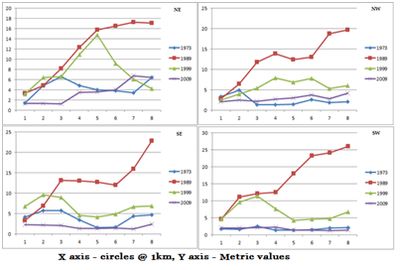
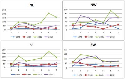
7.2 Shimoga: Number of Patches (NP) NP reflects the extent of fragmentation of a particular class in the landscape. Higher the value more the fragmentation, Lower values is indicative of clumped patch or patches forming a single class. The results (figure 11a) show that center is in the verge of clumping especially accelerated in 2005 and 2010, while the outskirts remain fragmented and are highly fragmented during 2005 and 2010 in North east, south east and south west directions. North west zone is losing its vegetation and cultivation class and this zone is highly fragmented in the outskirts during 2005 but is now in the verge of forming a single built up class.
Largest patch index: LPI (figure 11b) indicates that the landcape is aggregating to form single patches in almost all directions and gradients. Fragmented outskirts are also now on the verge of forming a single patch, and core center is almost constant except in north east and south east directions as it has also water class which is comparatively a large patch .
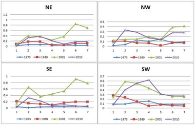
Patch Density (PD): PD refers to number of patches per unit considered. This index is computed using a raster data with4 neighbour algorithm. Patch density increases with a greater number of patches within a reference area. As seen before the fragmentation is large in the buffer regions and hence the patch density is high in the buffer region as compared to the core area. Patch density increased with number of patches increasing in mid-90’s further continued till 2005. During the years 2005- 2010 patch density considerably decreased as number of patches decreased and hence indicated the process of clumping. Figure 11c explains the patch density at patch level.
Normalized Landscape Shape Index (NLSI): NLSI calculates the value based on particular class rather than landscape and is equal to zero when the landscape consists of single square or maximally compact almost square, its value increases when the patch types becomes increasingly disaggregated and is 1 when the patch type is maximally disaggregated. The results (Figure 11d) indicate that the urban area is almost clumped in all direction and all gradients especially in north east and west direction. It shows a small degree of fragmentation in the buffer regions in south west and south east direction. The core area is in the process of becoming maximally square in all directions.
Interspersion and Juxtaposition (IJI): Interspersion and Juxtaposition approaches 0 when the distribution of adjacencies among unique patch types becomes increasingly uneven. IJI is equal to 100 when all the patch types are equally adjacent to all other patch types. Analysis on the study region indicates (Figure 11e) that near the core the values are near zero indicating adjacencies are uneven whereas in the outskirts and buffer zones values are relatively higher indicating that they are relatively adjacent and clumped
| Fig 11a: Number of patches (zonewise, circlewise) | Fig 11b: Largest Patch – zonewise, circlewise |
| Fig 11c: Patch density – zonewise, circle wise | Figure 11d: Zonewise and circle wise NLSI |
| Figure 11e: IJI Index | |
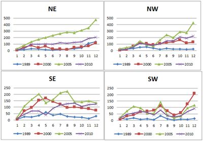
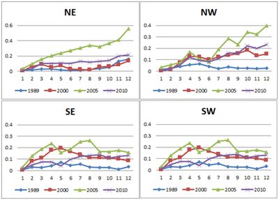
7.3 Hubli-Dharwad: Figure 12a illustrates that the Hubli city is forming patched that are clumped at the center but is relatively disaggregated at the outskirts, but compared to the year 2005, 2010 results is indicative of clumped urban patch in the city and is directive of forming a single urban patch. Clumped patches are more prominent in NE and SW directions and patches is agglomerating to a single urban patch. The case with Dharwad is different as in case it has started to disaggregate in 2010, until 2010 there were less no of urban patches in the city, which have increased in 2010, which is indicative of sprawled growth in the city.
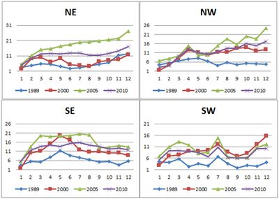
Patch density (Fig 12b) is calculated on a raster map, using a 4 neighbor algorithm. Patch density increases with a greater number of patches within a reference area.Patch density in Hubli and Dharwad was higher in 2005 as the number of patches is higher in all directions and gradients due to increase in the urban built area, which remarkably increased post 1989(SW, NE) and subsequently reduced in 2010, indicating the sprawl in the region in in early 90’s and started to clump during 2010. The patch density is quite high in the outskirts also in both the cities.
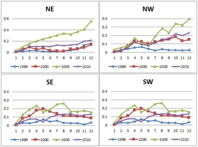
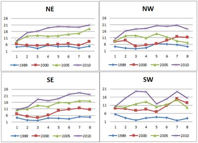
Landscape Shape Index (LSI): LSI equals to 1 when the landscape consists of a single square or maximally compact (i.e., almost square) patch of the corresponding type and LSI increases without limit as the patch type becomes more disaggregated. Results (Fig 12c) indicate that there were low LSI values in 1989 as there was minimal urban areas in both Hubli and Dharwad which were mainly aggregated at the center. Since late 1990’s both the city has been experiencing dispersed growth in all direction and circles and Hubli reached the peak of dispersed growth during 2005, towards 2010 it shows a aggregating trend in Hubli, whereas In Dharwad it is showing an dispersed growth.
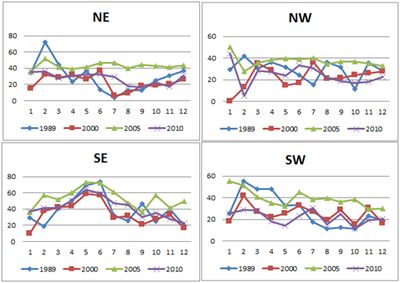
Percentage of Like Adjacencies (Pladj) is the percentage of cell adjacencies involving the corresponding patch type those are like adjacent. Cell adjacencies are tallied using the double-count method in which pixel order is preserved, at least for all internal adjacencies. This metrics also explains the adjacencies of urban patches that the city center is getting more and more clumped with similar class (Urban) and outskirts are relatively sharing different internal adjacencies. Hubli city shows more adjacent clumped growth, whereas Dharwad shows more disaggregated growth (Fig. 12d).
 Hubli |
 Dharwad |
| Figure 12a: Number of urban patches (Directionwise, circlewise) | |
 Hubli |
 Dharwad |
| Figure 12b: Patch Density (Directionwise, circlewise) | |
 Hubli |
 Dharwad |
| Figure 12c: Landscape Shape Index (Directionwise, circlewise) | |
 Hubli |
 Dharwad |
| Figure 12d: Percentage of Like Adjacencies (Direction wise, circle wise) | |
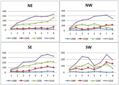
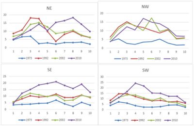
7.4 Gulbarga: Number of patches: Figure 13a illustrates of the urban growth evident from the increase in number of patches in 1992 and 2002 whereas in 2010 the patches have decreased indicating aggregation or clumped growth, while outskirts and boundary area (5thcircle onwards) is showing a fragmented growth. Clumped patches at center are more prominent in NE and SE directions. Outskirts are fragmented more in NE and SE directions indicative of higher sprawl in the region.
The patch density (Figure 13b) is calculated on a raster data, using a 4 neighbour algorithm. Patch density increases with a greater number of patches within a reference area. Patch density was higher in 1992 in all directions and gradients due to small urban patches. This remarkably increased in 2002 in the outskirts which are an indication of sprawl in 2002, subsequently increasing in 2010. PD is low at centre indicating the clumped growth, which was in accordance with number of patches.
Landscape Shape Index (LSI): LSI equals to 1 when the landscape consists of a single square or maximally compact (i.e., almost square) patch of the corresponding type and LSI increases without limit as the patch type becomes more disaggregated. Figure 6c indicates of lower LSI values in 1973 due to minimal concentrated urban areas at the center. The city has been experiencing dispersed growth in all direction and circles since 1990’s. In 2010 it shows a aggregating trend at the centre as the value is close to 1, whereas it is very high in the outskirts indicating the peri urban development (fig 13c).
Patch cohesion index measures the physical connectedness of the corresponding patch type. This is sensitive to the aggregation of the focal class below the percolation threshold. Patch cohesion increases as the patch type becomes more clumped or aggregated in its distribution; hence, more physically connected. Above the percolation threshold, patch cohesion is not sensitive to patch configuration. Figure 13d indicate of physical connectedness of the urban patch with the higher cohesion value (in 2010). Lower values in 1973 illustrate that the patches were rare in the landscape.
 |
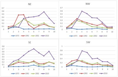 |
| Fig 13a: Number of urban patches (zonewise, circlewise) | Fig 13b: Patch density – zonewise, circle wise |
 |
 |
| Fig 13c: Landscape Shape Index | Figure 13d: Zonewise and circle wise Patch cohesion |
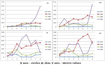
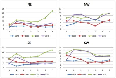
7.5 Raichur: Number of patches: Figure 14a illustrates the temporal dynamics of number of patches. Urban patches are less at the center in 1970’s as the growth was concentrated in central pockets. There was a gradual increase in the number of patches in 80’s and further in 2001, but these patches are forming a single patch during 2010 indicative that the urban area is getting clumped as a single patch at the center, but in the buffer regions there has been a tremendous increase in 2001. Clumped patches at center are more prominent in NE and SE directions and patches is agglomerating to a single urban patch.
The patch density (Fig 14b) is calculated on a raster map, using a 4 neighbor algorithm. Patch density increases with a greater number of patches within a reference area. Patch density was higher in 1989 and 2001 as the number of patches is higher at the in all directions. Ensity declined at the central gradients in 2010. In the outskirts the patch density has increased in early 2000’s which is indicative of sprawl in the region and PD is low at center indicating the clumped growth during late 2000’s, which was in accordance with number of patches.
Landscape Shape Index (LSI): LSI equals to 1 when the landscape consists of a single square or maximally compact (i.e., almost square) patch of the corresponding type and LSI increases without limit as the patch type becomes more disaggregated. Results (Fig 14c) indicate that there were low LSI values in 1973 as there were minimal urban areas and were concentrated in the center. Since 1990’s the city has been experiencing dispersed growth in all direction and circles, towards 2010 it shows a aggregating trend at the center as the value is close to 1, whereas it is very high in the outskirts indicating the peri urban development.
Patch cohesion index measures the physical connectedness of the corresponding patch type. Figure 14d indicate of physical connectedness of the urban patch with the higher cohesion value (in 2010). Lower values in 1973 illustrate that the patches were rare in the landscape.
 |
 |
| Fig 14a: Number of patches index (zonewise, circlewise) | Fig 14b: Patch density – zonewise, circle wise |
 |
 |
| Fig 14c: Landscape shape index – zonewise, circle wise | Figure 14d: Zonewise and circle wise Patch cohesion |
7.6 Bellary: Number of Urban Patch (Np) is a landscape metric indicates the level of fragmentation and ranges from 0 (fragment) to 100 (clumpiness). Figure 15a illustrates the temporal dynamics of number of patches. Increased number of patches indicates the land fragmentation and decreasing of increased patches indicates the fragmented landscape forming a single land use patch. As observed from the figure, urban patches are least in the landscape in 1970’s as the growth was concentrated on at the city center. In 2000’s Bellary city saw a gradual increase in the number of patches, which can be understood as features of fragmented landscape, further in 2010, these patches are increasingly forming a single patch at the center during 2010 indicative that the urban area forming a single clump patch destroying all other land uses, but the case in the buffer regions has been indicative of higher fragmentation during the latter years. Clumped patches at center are more prominent in NE and SE directions and patches are agglomerating to a single urban patch.
Landscape Shape Index (LSI): LSI equals to 1 when the landscape consists of a single square or maximally compact (i.e., almost square) patch of the corresponding type and LSI increases without limit as the patch type becomes more disaggregated. Results (Fig 15b) indicate that there were low LSI values in 1973 as there were minimal urban areas and were concentrated in the center. Since 2001 the city has been experiencing dispersed growth in all direction and in every gradient, towards 2010 it shows aggregating urban land use at the center forming a simple shaped single patch as the value is close to 1, whereas, the values of LSI are very high in the outskirts indicating a complex shaped growth with also is indicative of fragmented landscape in the buffer zone.
Largest Patch Index (LPI): This metric reveals information about the largest patches in the Landscape and its native existence. Urban patch again counted as a largest patch in 2010 in the central area of Bellary, whereas the buffer zones had a mixture of other patches. Figure 15c is illustrative of results of this analysis.
Patch cohesion index measures the physical connectedness of the corresponding patch type. Figure 15d describes the results of the analysis of physical connectedness of the urban patch with the higher cohesion value (in 2010) indicating that the urban count is higher in the considered study region. Lower values in 1973 illustrate that the urban patches were rare in the landscape.
 |
 |
| Fig 14a: Number of patches index (zonewise, circlewise) | Fig 14b: Patch density – zonewise, circle wise |
 |
|
| Fig 14c: Landscape patch index – zonewise, circle wise | Figure 14d: Zonewise and circle wise Patch cohesion |
7.7 Belgaum: Number of Patches (NP): NP is a type of metric describes the growth of particular patches wither in a aggregated or fragmented patch growth in the region and also explains the underlying urbanization process. Number of Patch is always equal to or greater 1, NP = 1 indicates that there is only 1 patch of a particular class, showing aggregated growth, larger values of NP indicate fragmented growth. The results indicate that there has been an extensive growth of urban patches in all directions post 2000, which have increased specially in the buffer zones, which indicate the growth of sprawl area as fragments represented in figure 15a.
Patch Density (PD): PD is a landscape metric which is quite similar to number of patches but gives density about the landscape in analysis, The values vary from 0 to 1, 0 indicating a single homogenous patch, whereas values towards 1 indicates fragmented growth as the patches increase the patch density increases. The results as observed that from the figure 15b below, the landscape under study is becoming fragmented towards the outskirts, but at the core of the city, clumped patches are prominent in all directions specially post 2000. In 2012, this substantially decreased in almost all directions mainly due to patches getting clumped and forming a single patch.
Landscape Shape Index (LSI): LSI provides a measure of class aggregation or clumpiness depending on the shape of the class in analysis, when the value of LSI is 1, this indicates clumped growth, the increasing values of LSI indicates aggregation. Figure 15c represents the results of LSI. The results of metric puts out a fact that in 2012 landscape class shapes are becoming more complex indicative of fragmented growth, with comparison of simple shape in 1980’s a clumped growth
Cohesion measures the physical connectivity between adjacent patches; the cohesion value 0 indicates disaggregation and no inter connectivity between patches and higher value indicates clumped and connectivity between patches. Value higher post 2000 tells us that the fragmented landscape if forming a single clumped patch.in almost all gradients and zones (Figure 15d).
 |
 |
| Fig 15a: Number of patches index (zonewise, circlewise) | Fig 15b: Patch density – zonewise, circle wise |
 |
|
| Fig 15c: Landscape shape index – zonewise, circle wise | Figure 15d: Zonewise and circle wise Patch cohesion |