|
Results
Land Cover Analysis: To understand the spatial extent of area under vegetation and non-vegetation, various land cover indices were analyzed. Among these NDVI index provide better insights to understand the extent of vegetation cover. Temporal NDVI were calculated and the results are given in Fig. 4 and in Table IV. The results indicate that the vegetation in the study region decreased for 98.8% (in 1989) to 91.74% (in 2012). Further temporal land use analyses are done to understand the changes in land uses.
Table IV. Land cover analysis
| Year |
Vegetation |
Non Vegetation |
| 1989 |
98.8% |
1.2% |
| 2000 |
98.41% |
1.59% |
| 2006 |
96.35% |
3.65% |
| 2012 |
91.74 % |
8.26 % |
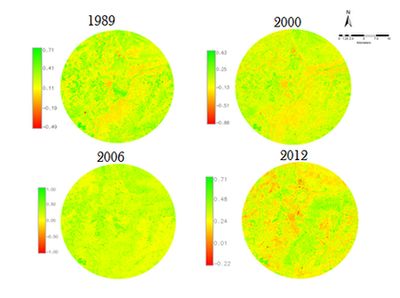
Figure. 4. Land Cover Classification
Land Use Analysis: Temporal land use changes during 1989 to 2012 were analysed. Spatial data were analysed using maximum likelihood Classifier and the results are shown in Fig. 5 and Table V. The results of the analysis indicate that the urban impervious land use has increased from 0.31 % (in 1989) to 6.74% (in 2012); vegetation decreased from 4.62% (in 1989) to 2.44% (in 2012), while water category remained fairly constant.
Table V. Land Use analysis
| Year |
1989 |
2000 |
| Land use |
% |
Area(Ha) |
% |
Area(Ha) |
| Water |
0.14 |
53.24 |
0.33 |
125.49 |
| Vegetation |
4.62 |
1756.92 |
2.58 |
981.14 |
| Built up |
0.31 |
117.89 |
1.17 |
444.93 |
| Others |
94.9 |
36089.11 |
95.92 |
36477.00 |
| Year |
2006 |
2012 |
| Land use |
% |
Area(Ha) |
% |
Area(Ha) |
| Water |
0.23 |
87.47 |
0.24 |
92.03 |
| Vegetation |
2.33 |
886.07 |
2.44 |
928.73 |
| Built up |
4.81 |
1829.17 |
6.74 |
2190.15 |
| Others |
92.93 |
35339.95 |
91.58 |
34904.41 |
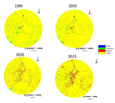
Fig.5. Land Use Classification
Accuracy Assessment and Kappa Statistics: Kappa Statistics serves as an indicator of the extent pixels are correctly classified into the respective categories. The accuracy assessment was carried out for the classified data and the results are given in Table VI. The results indicated that the accuracy was above 90% and kappa values had strong agreement with the accuracy values with an average of 0.9.
Table VI. Accuracy assessment
| Year |
Overall Accuracy |
Kappa Value |
| 1989 |
94.85 |
0.87 |
| 2000 |
92.73 |
0.83 |
| 2006 |
93.64 |
0.92 |
| 2012 |
93.12 |
0.93 |
Urbanisation analysis using Shannon’s entropy:Shannon entropy, as an indicator of urban sprawl was calculated and the results are shown in Fig. 6 and Table VII. The threshold limit of Shannon’s Entropy is log11 or 1.041. The results indicated that though Belgaum and the buffer region is not experiencing urban sprawl. However increasing entropy values show the tendency of sprawl in the region.
Table VII. Built Up and Shannon’s Entropy Analysis
| Year |
NE |
NW |
SE |
SW |
| 1989 |
0.0059 |
0.0191 |
0.0034 |
0.0088 |
| 2000 |
0.0283 |
0.0546 |
0.017 |
0.0334 |
| 2006 |
0.0791 |
0.140 |
0.108 |
0.113 |
| 2012 |
0.0864 |
0.1652 |
0.1154 |
0.137 |
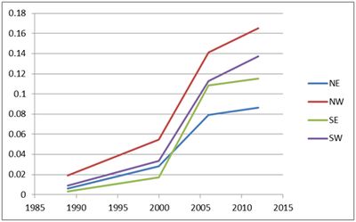
Figure.6. Shannon Entropy
5.6 Spatial patterns analysis:Spatial patterns of the landscape was analysed considering metrics based on the urban land use changes. Various landscape metrics were calculated as discussed.
Proportion of Landscape (PLAND): PLAND indicates the percentage of urban land present in particular gradient and zone and ranges from 0 to 1, the value 1 indicates the landscape comprises of a single urban class and zero represents absence of urban class. The results of the analysis are represented in Fig. 7a, which indicates spurt in urban land use during post 2000 and especially in 2012 in almost all directions and all gradients.
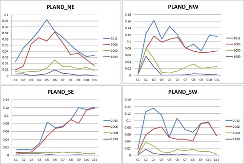
X axis : Circles at every 1 km, Y axis: Indices value
Figure. 7a:Proportion of landscape metric
Number of Patches (NP): NP is a type of metric describes the growth of particular patches whether in an aggregated or fragmented growth in the region and also explains the underlying urbanization process. Number of Patch is always equal to or greater 1, NP = 1 indicates that there is only 1 patch of a particular class, showing aggregated growth, larger values of NP indicate fragmented growth. The results indicate that there growth of urban patches in all directions post 2000, which have increased specially in the buffer zones, due to fragments as in Fig. 7b.
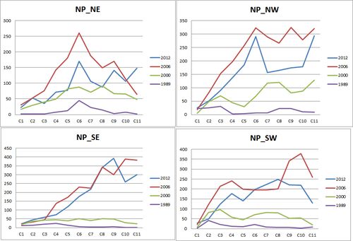
X axis: Circles at every 1 km, Y axis: Index value
Figure.7b. Number of patches metric analysed.
Patch Density (PD): PD is a landscape metric which is quite similar to number of patches but gives density about the landscape in analysis, The values vary from 0 to 1, 0 indicating a single homogenous patch, whereas values towards 1 indicates fragmented growth as the patches increase the patch density increases. The results as in Fig. 7c indicates an increase of NP in the outskirts, but at the core of the city, clumped patches are prominent in all directions specially post 2000. In 2012, this substantially decreased in almost all directions mainly due to patches getting clumped and forming a single patch.
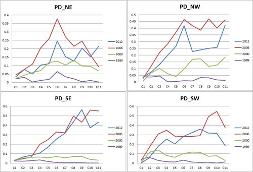
X axis: Circles at every 1 km, Y axis: Indices value
Figure.7c. Patch density metric
Total Edge (TE) and Edge density (ED): TE is the absolute measure of total length (perimeter) of each class of a particular patch in landscape in meters. TE considers true edges into consideration. Value of TE is greater than or equal to zero. Larger the edge values indicate larger continuous patches. ED is the ratio of total edge distance to the total Area. If ED is zero, it represents there is no class of the landscape. Fig. 7d explains the results of the analysis, which indicate that during 1980’s the edges were smaller, which explains that the urban patch was rare in landscape and was concentrated, but post 2000 +and in 2012 there are larger edges, which indicate that the urban area is continuous. This phenomenon is true in the city boundary, but the buffer region patches are yet fragmented and non-continuous. Fig. 7e explains the edge density which has the agreement with the metrics explained earlier, indicative of the fragmented patches becoming a single patch in 2012
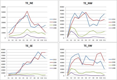
X axis: Circles at every 1 km, Y axis: Index value
Figure. 7d: Total Edge metric
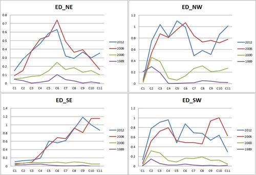
X axis: Circles at every 1 km, Y axis: Index value
Figure.7e. Edge Density metric
Landscape Shape Index (LSI) and Normalized Landscape Shape Index(NLSI): LSI provides a measure of class aggregation or clumpiness depending on the shape of the class in analysis, when the value of LSI is 1, this indicates clumped growth, the increasing values of LSI indicates aggregation. NLSI is the normalized value of LSI, when zero or closer to zero indicates a clumped growth whereas NLSI towards 1 indicates aggregated growth of the landscape. Fig. 7f and 7g represents the results of LSI and NLSI. The results of both metrics puts out a fact that in 2012 landscape class shapes are becoming more complex indicative of fragmented growth, with comparison of simple shape in 1980’s a clumped growth
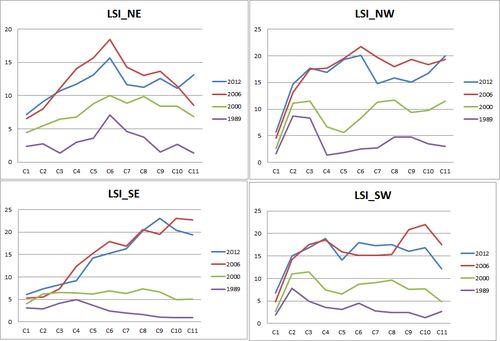
X axis: Circles at every 1 km, Y axis: Indices value
Figure.7f. Landscape Shape Index metric
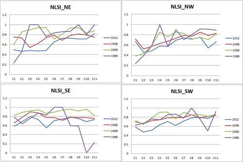
X axis: Circles at every 1 km, Y axis: Indices value
Figure. 7g. Normalised Landscape Shape Index metric
Fractal Dimension Index represents the complexity of the shape of the landscape. The values vary from 1 to 2; index values closer to 1 indicates simpler shapes of the land scape values closer to 2 indicate varying shape of the landscape. Fig. 7h explains that the complexity of shape increases in 2012 when compared to 1989 accompanied with simple shapes and perimeters.
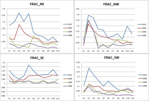
X axis: Circles at every 1 km, Y axis: Indices value
Figure.7h. Fractal Dimension Metrics in four directions
Contiguity indicates the continuity of the landscape, Contiguity index varies from 0 to 1, values closer to zero indicates single pixel, values closer to one indicates patch with large number of pixels of the particular class. Fig. 7i explains the output of the contiguity metric, explaining the dominance of the urban pixels in all directions post 2000, which was less in 1980’s.
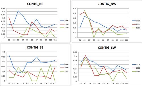
X axis: Circles at every 1 km, Y axis: Indices value
Figure.7i. Contiguity metric
Cohesion measures the physical connectivity between adjacent patches; the cohesion value 0 indicates disaggregation and no inter connectivity between patches and higher value indicates clumped and connectivity between patches. Higher values during post 2000 illustrate of fragmented landscape forming clumped patches in almost all gradients and zones (Fig. 7j).
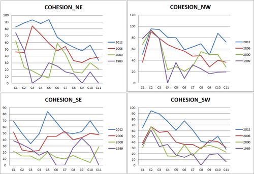
X axis: Circles at every 1 km, Y axis: Indices value
Figure.7j. Cohesion Metric
Aggregation index is a measure of disaggregation or aggregation of a landscape, the metric varies from zero to 100 percent, values closer to zero indicate disaggregation and values closer to 100 indicate aggregated growth of the landscape. Fig. 7k corroborates with the earlier metrics that post 1980’s the landscape had been fragmented which has started aggregating during post 2000.
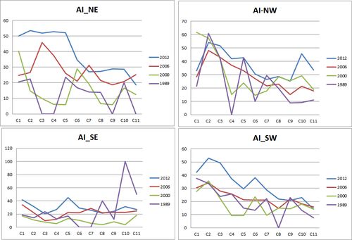
X axis: Circles at every 1 km, Y axis: Indices value
Figure.7k. Aggregation Index
|
