|
Method
A three-step approach as illustrated in Fig. 2 was adopted to understand the dynamics of the urbanizing city, which includes (i) a normative approach to understand the LULC dynamics (ii) a gradient approach of 1km radius to understand the pattern of growth during the past four decades. (iii) Quantifying the growth over time using spatial metrics. Various stages in the data analysis are
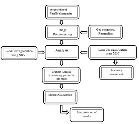
Figure 2. Procedure followed to understand the spatial pattern of landscape change
4.1 Preprocessing: The remote sensing data of Landsat were downloaded from GLCF (Global Land Cover Facility, http://glcf.umiacs.umd.edu/data) and IRS LISS III data were obtained from NRSC, Hyderabad (http://nrsc.gov.in). The data obtained were geo-referenced, rectified and cropped pertaining to the study area. Landsat data has a spatial resolution of 28.5 m x 28.5 m (nominal resolution) were resampled to uniform 30 m for inter temporal data comparisons.
4.2 Vegetation Cover Analysis: Vegetation cover analysis was performed using the index Normalized Difference Vegetation index (NDVI) was computed for all the years to understand the change in the temporal dynamics of the vegetation cover in the study region. NDVI value ranges from values -1 to +1, where -0.1 and below indicate soil or barren areas of rock, sand, or urban built-up. NDVI of zero indicates the water cover. Moderate values represent low density vegetation (0.1 to 0.3) and higher values indicate thick canopy vegetation (0.6 to 0.8).
4.3 Land use analysis: Further to account for changes in the landscape, land use analysis were performed and categories considered are listed in Table II.
Table II: Land use categories
| Land use Class |
Land uses included in the class |
| Urban |
This category includes residential area, industrial area, and all paved surfaces and mixed pixels having built up area. |
| Water bodies |
Tanks, Lakes, Reservoirs. |
| Vegetation |
Forest, Cropland, nurseries. |
| Others |
Rocks, quarry pits, open ground at building sites, kaccha roads. |
Data were classified with the training data (field data) using Gaussian maximum likelihood supervised classifier. Analysis involved i) generation of False Colour Composite (FCC) of remote sensing data (bands – green, red and NIR). This helped in locating heterogeneous patches in the landscape ii) selection of training polygons (these correspond to heterogeneous patches in FCC) covering 15% of the study area and uniformly distributed over the entire study area, iii) loading these training polygons co-ordinates into pre-calibrated GPS and collection of the corresponding attribute data (land use types) for these polygons from the field. GPS helped in locating respective training polygons in the field, iv) supplementing this information with Google Earth (http://www.googleearth.com) and Bhuvan (http://bhuvan.nrsc.gov.in) v) 60% of the training data has been used for classification, while the balance is used for validation or accuracy assessment.
Gaussian maximum likelihood classifier (GMLC) is used to classify the data using the training data. GMLC uses various classification decisions using probability and cost functions [28] and is proved superior compared to other techniques. Mean and covariance matrix are computed using estimate of maximum likelihood estimator. Estimations of temporal land uses were done through open source GIS (Geographic Information System) - GRASS (Geographic Resource Analysis Support System, http://ces.iisc.ac.in/grass). 70% of field data were used for classifying the data and the balance 30% were used in validation and accuracy assessment. Thematic layers were generated of classifies data corresponding to four land use categories.
Evaluation of the performance of classifiers is done through accuracy assessment techniques of testing the statistical significance of a difference, comparison of kappa coefficients and proportion of correctly allocated classes (Jensen, 2005) through computation of confusion matrix. These are most commonly used to demonstrate the effectiveness of the classifiers (3,18,29,30). Further each zone was divided into concentric circle of incrementing radius of 1 km (Fig. 3) from the center of the city for visualising the changes at neighborhood levels. This also helped in identifying the causal factors and the degree of urbanization (in response to the economic, social and political forces) at local levels and visualizing the forms of urban sprawl. The temporal built up density in each circle is monitored through time series analysis.
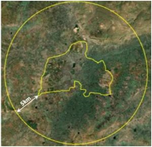
Figure 3. Study Area with 5 Km Buffer Overlaid on Spatial Data (Google Earth)
Urban sprawl analysis: Direction-wise Shannon’s entropy (Hn) is computed (equation 1) to understand the extent of growth: compact or divergent (30,10). This provides an insight into the development (clumped or disaggregated) with respect to the geographical parameters across ‘n’ concentric regions in the respective zones.
 …… (1) …… (1)
Where Pi is the proportion of the built-up in the ith concentric circle and n is the number of circles/local regions in the particular direction. Shannon’s Entropy values ranges from zero (maximally concentrated) to log n (dispersed growth).
Spatial pattern analysis: Spatial metrics provide quantitative description of the composition and configuration of urban landscape. These metrics were computed for each circle, zonewise using classified land use data at the landscape level with the help of FRAGSTATS [31]. Urban dynamics is characterised by prominent spatial metrics chosen based on Shape, edge, complexity, and density criteria. The metrics include the patch area, shape, epoch/contagion/ dispersion and are listed in Table III.
Table III. Landscape metrics analysed
| |
Indicators |
Formula |
| 1 |
Number of Urban Patches (NPU) |
NPU = n
NP equals the number of patches in the landscape. |
| 2 |
Patch density(PD) |
f(sample area) = (Patch Number/Area) * 1000000 |
| 3 |
Normalized Landscape Shape Index (NLSI) |
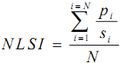
Where siand pi are the area and perimeter of patch i, and N is the total number of patches. |
| 4 |
Landscape Shape Index (LSI) |

ei =total length of edge (or perimeter) of class i in terms of number of cell surfaces; includes all landscape boundary and background edge segments involving class i.
minei=minimum total length of edge (or perimeter) of class i in terms of number of cell surfaces. |
| 5 |
Total Edge (TE) |
 , ,
where, eik = total length (m) of edge in landscape involving patch type (class) i; includes landscape boundary and background segments involving patch type i. |
| 6 |
Percentage of Land (Pland) |
 , ,
Pi = proportion of the landscape occupied by patch type (class) i. aij = area (m2) of patch ij, A =total landscape area (m2). |
| 7 |
Aggregation index(AI) |
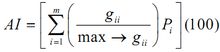
gii =number of like adjacencies between pixels of patch type
Pi= proportion of landscape comprised of patch type. |
| 8 |
Cohesion |
pij = perimeter of patch ij in terms of number of cell surfaces.
aij = area of patch ij in terms of number of cells.
A = total number of cells in the landscape |
| 9 |
Edge Density (ED) |
eik = total length (m) of edge in landscape involving patch type (class) i; includes landscape boundary and background segments involving patch type i. A =total landscape area (m2). |
| 10 |
Contiguity Index |
cijr =contiguity value for pixel r in patch ij.
v = sum of the values in a 3-by-3 cell template (13 in this case).
aij = area of patch ij in terms of number of cells |
| 11 |
Area weighted mean Fractal index |
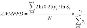 |
|
