 |
Status of Wetlands in Urbanising Tier II cities of Karnataka: Analysis using Spatio Temporal data |
 |
1Energy and Wetlands Research Group, Centre for Ecological Sciences [CES],
2Centre for Sustainable Technologies, 3Centre for infrastructure, Sustainable Transportation and Urban Planning (CiSTUP),
Indian Institute of Science, Bangalore – 560012, India.
*Corresponding author: cestvr@ces.iisc.ac.in
|
Materials used
The time series spatial data acquired from Landsat MSS (57.5), Landsat Series Thematic mapper (28.5m) sensors for the temporal period were downloaded from public domain (http://glcf.umiacs.umd.edu/data). IRS LISS III (24 m) data coinciding with the field investigation dates were procured from National Remote Sensing Centre (www.nrsc.gov.in), Hyderabad. Survey of India (SOI) topo-sheets of 1:50000 and 1:250000 scales were used to generate base layers of city boundary, etc. Table1 lists the data used in the current analysis. Ground control points to register and geo-correct remote sensing data were collected using handheld pre-calibrated GPS (Global Positioning System), Survey of India Toposheet and Google earth (http://earth.google.com, http://bhuvan.nrsc.gov.in).
Table I: Data used for the analysis
| DATA |
Purpose |
| Landsat Series MSS(57.5m) |
Land cover and Land use analysis |
| Landsat Series TM (28.5m) and ETM |
Land cover and Land use analysis |
| IRS LISS III (24m) |
Land cover and Land use analysis |
| Survey of India (SOI) toposheets of 1:50000 and 1:250000 scales |
To Generate boundary and Base layer maps. |
| Field visit data –captured using GPS |
For geo-correcting and generating validation dataset |
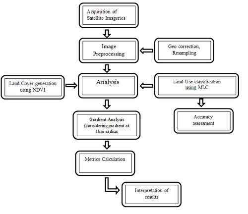
Figure 2: Procedure followed to understand the spatial pattern of landscape change
Method
A two-step approach was adopted to chart the direction of the City’s development, which includes (i) a normative approach to understand the land use and (ii) a gradient approach of 1km radius to understand the pattern of growth during the past 4 decades. Various stages in the data analysis are
-
Preprocessing: The remote sensing data obtained were geo-referenced, rectified and cropped pertaining to the study area. The Landsat satellite MSS images have a spatial resolution of 57.5 m x 57.5 m (nominal resolution) and landsat TM and landsat ETM (1989 -2010) data of 28.5 m x 28.5 m (nominal resolution) were resampled to uniform 30 m for intra temporal comparisons. Data in case of non-availability of landsat data, IRS LISS3 of spatial resolution 24 m was procured from NRSC, Hyderabad (http://www.nrsc.gov.in) also was resampled to 30m.
-
Vegetation Cover Analysis: Normalised Difference Vegetation index (NDVI) was computed to understand the temporal dynamics of the vegetation cover. NDVI value ranges from values -1 to +1, where -0.1 and below indicate soil or barren areas of rock, sand, or urban builtup. NDVI of zero indicates the water cover. Moderate values represent low density vegetation (0.1 to 0.3) and higher values indicate thick canopy vegetation (0.6 to 0.8).
-
Land use analysis: Land use categories listed in Table 2 were classified with the training data (field data) using Gaussian maximum likelihood supervised classier. The analysis included generation of False Color Composite (bands – green, red and NIR), which helped in identifying heterogeneous area. Polygons were digitized corresponding to the heterogeneous patches covering about 40% of the study region and uniformly distributed over the study region. These training polygons were loaded in pre-calibrated GPS (Global position System). Attribute data (land use types) were collected from the field with the help of GPS corresponding to these polygons. In addition to this, polygons were digitized from Google earth (www.googleearth.com) and Bhuvan (bhuvan.nrsc.gov.in), which were used for classifying latest IRS P6 data. These polygons were overlaid on FCC to supplement the training data for classifying landsat data.
Table II: Land use categories
| Land use Class |
Land uses included in the class |
| Urban |
This category includes residential area, industrial area, and all paved surfaces and mixed pixels having built up area. |
| Water bodies |
Tanks, Lakes, Reservoirs. |
| Vegetation |
Forest, Cropland, nurseries. |
| Others |
Rocks, quarry pits, open ground at building sites, kaccha roads. |
Gaussian maximum likelihood classifier (GMLC) is applied to classify the data using the training data. GMLC uses various classification decisions using probability and cost functions (Duda et al., 2000) and is proved superior compared to other techniques. Mean and covariance matrix are computed using estimate of maximum likelihood estimator. Estimations of temporal land uses were done through open source GIS (Geographic Information System) - GRASS (Geographic Resource Analysis Support System, http://ces.iisc.ac.in/grass) which is the world biggest open source software project. 70% of field data were used for classifying the data and the balance 30% were used in validation and accuracy assessment. Thematic layers were generated of classifies data corresponding to four land use categories.
Further each zone was divided into concentric circle of incrementing radii of 1 km from the center of the city for visualising the changes at neighborhood levels. This also helped in identifying the causal factors and the degree of urbanization (in response to the economic, social and political forces) at local levels and visualizing the forms of urban sprawl. The temporal built up density in each circle is monitored through time series analysis.
-
Urban sprawl analysis: Direction-wise Shannon’s entropy (Hn) is computed (equation 1) to understand the extent of growth: compact or divergent (Sudhira et al., 2004, Ramachandra et al., 2012). This provides an insight into the development (clumped or disaggregated) with respect to the geographical parameters across ‘n’ concentric regions in the respective zones.
 …… (1) …… (1)
Where Pi is the proportion of the built-up in the ith concentric circle and n is the number of circles/local regions in the particular direction. Shannon’s Entropy values ranges from zero (maximally concentrated) to log n (dispersed growth).
Spatial pattern analysis: Landscape metrics provide quantitative description of the composition and configuration of urban landscape. These metrics were computed for each circle, zone wise using classified land use data at the landscape level with the help of FRAGSTATS an open source software. Urban dynamics is characterised by 3 spatial metrics chosen based on complexity and density criteria. The metrics include the patch area, edge/border, shape, epoch/contagion/ dispersion and are listed in Table III.
Table III: Spatial Landscape Indices
| |
Indicators |
Formula |
Range |
| 1 |
Number of Urban Patches (NPU) |

NP equals the number of patches in the landscape. |
NPU>0, without limit. |
| 2 |
Normalized Landscape Shape Index (NLSI) |

Where si and pi are the area and perimeter of patch i, and N is the total number of patches. |
0≤NLSI<1 |
| 3 |
Clumpiness |

Pi =proportion of the landscape occupied by patch type (class) i. |
-1≤ CLUMPY ≤1. |
|
|
Citation : Bharath H. Aithal, Durgappa S. and Ramachandra. T.V, 2012. Status of Wetlands in Urbanising Tier II cities of Karnataka: Analysis using Spatio Temporal data., Proceedings of the LAKE 2012: National Conference on Conservation and Management of Wetland Ecosystems, 06th - 09th November 2012, School of Environmental Sciences, Mahatma Gandhi University, Kottayam, Kerala, pp. 1-12.
|