|
Spatio temporal patterns of urban growth in Bellary, Tier II City of Karnataka State, India
|
 |
1Energy & Wetlands Research Group, Centre for Ecological Sciences [CES], 2Centre for Sustainable Technologies (astra), 3Centre for infrastructure, Sustainable Transportation and Urban Planning [CiSTUP],
Indian Institute of Science, Bangalore – 560012, India.
*Corresponding author: cestvr@ces.iisc.ac.in
|
MATERIALS AND METHODS
Urban dynamics has been assessed using remote sensing data of the period 1989 to 2010. Time series spatial data acquired from Landsat Series Thematic mapper (28.5m) sensors for the period 1989 and 2000were downloaded from public domain [23], IRS LISS III data (24 m) for 2005 and 2010 were procured from the National remote Sensing Centre [24], Hyderabad. Survey of India (SOI) toposheets of 1:50000 and 1:250000 scales were used to generate base layers of city boundary, etc. City map with ward boundaries were digitized from the city administration map. Population data was collected from the Directorate of Census Operations, Bangalore region [21]. Table I lists the data used in the current analysis. Ground control points to register and geo-correct remote sensing data were collected using hand held pre-calibrated GPS (Global Positioning System), Survey of India toposheets (1:50000, 1:250000 scale), and virtual spatial maps - Google earth and Bhuvan ([22], [20]). See table1.
Table 1. Materials used in Analysis
| DATA |
Year |
Purpose |
| Landsat Series TM (28.5m) and ETM |
1973 |
Land cover and Land use analysis |
| IRS LISS III (24m) |
2001,2005,2010 |
Land cover and Land use analysis |
| Survey of India (SOI) topo-sheet of 1:50000 and 1:250000 scales |
|
To generate base layer maps (city boundary, etc.). |
| Field visit data –captured using GPS |
|
For geo-correcting and generating validation dataset |
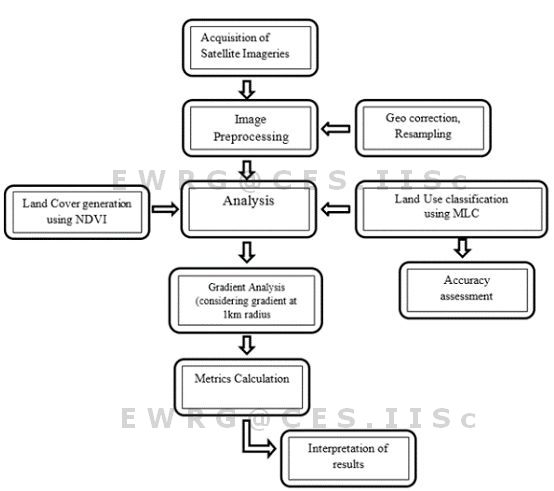
A three-step approach, illustrated in Figure 2 was adopted to understand the urban dynamics, which includes (i) a normative approach to understand the land use and land cover, (ii) a gradient approach of 1km radius to understand the pattern of growth during the past 4 decades, (iii) spatial metrics analysis for quantifying the growth. Various stages in the data analysis are:
- Preprocessing: The remote sensing data of landsat were downloaded from GLCF (Global Land Cover Facility) and IRS LISS III data were obtained from NRSC, Hyderabad. The data obtained were geo-referenced, rectified and cropped pertaining to the study area. The Landsat satellites have a spatial resolution of 28.5 m x 28.5 m (nominal resolution) were resampled to uniform 24 m for intra temporal comparisons.
- Vegetation Cover Analysis: Vegetation cover analysis was performed using the index Normalized Difference Vegetation index (NDVI) was computed for all the years to understand the temporal dynamics of the vegetation cover. NDVI values range from -1 to +1, where -0.1 and below indicate soil or barren areas of rock, sand, or urban built-up. NDVI of zero indicates the water cover. Moderate values represent low density vegetation (0.1 to 0.3) and higher values indicate thick canopy vegetation (0.6 to 0.8).
- Land use analysis: Further land use analysis was performed to investigate the changes in the landscape. Categories as listed in Table II, were classified with the training data (field data) using Gaussian maximum likelihood supervised classifier. The method involves i) generation of False Colour Composite (FCC) of remote sensing data (bands – green, red and NIR). This helped in locating heterogeneous patches in the landscape ii) selection of training polygons (these correspond to heterogeneous patches in FCC) covering 15% of the study area and uniformly distributed over the entire study area, iii) loading these training polygons co-ordinates into pre-calibrated GPS and collection of the corresponding attribute data (land use types) for these polygons from the field. GPS helped in locating respective training polygons in the field, iv) supplementing this information with Google Earth and Bhuvan v) 60% of the training data has been used for classification, while the balance is used for validation or accuracy assessment.
- Gaussian maximum likelihood classifier (GMLC) is applied to classify the remote sensing data of the study region using the training data. GMLC uses various classification decisions using probability and cost functions [39] and is proved superior compared to other techniques. Mean and covariance matrix are computed using estimate of maximum likelihood estimator. Estimations of temporal land uses were done through open source GIS (Geographic Information System) - GRASS (Geographic Resource Analysis Support System, http://ces.iisc.ac.in/grass). 60% of field data were used for classifying the data and the balance 40% were used in validation and accuracy assessment. Thematic layers were generated of classifies data corresponding to four land use categories (Table 2). Evaluation of the performance of classifiers is done through accuracy assessment techniques of testing the statistical significance of a difference, comparison of kappa coefficients and proportion of correctly allocated classes through computation of confusion matrix. These are most commonly used to assess the effectiveness of the classifiers ([37], [38]).
Figure 2: Procedure followed to understand the spatial pattern of landscape change
Table 2. Land use categories
| Land use Class |
Land uses included in the class |
| Urban |
This category includes residential area, industrial area, and all paved surfaces and mixed pixels having built up area. |
| Water bodies |
Tanks, Lakes, Reservoirs. |
| Vegetation |
Forest, Cropland, nurseries. |
| Others |
Rocks, quarry pits, open ground at building sites, kaccha roads. |
Further each zone was divided into concentric circle of incrementing radius of 1 km (figure 3) from the center of the city for visualising the changes at neighborhood levels. This also helped in identifying the causal factors and the degree of urbanization (in response to the economic, social and political forces) at local levels and visualizing the forms of urban sprawl. The temporal built up density in each circle is monitored through time series analysis.
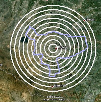
Figure 3. Google earth representation of Bellary
- Urban sprawl analysis: Direction-wise Shannon’s entropy (Hn) is computed (equation 1) to understand the extent of growth: compact or divergent ([27], [42], [40]). This provides an insight into the development (clumped or disaggregated) with respect to the geographical parameters across ‘n’ concentric regions in the respective zones.
 …… (1) …… (1)
Where Pi is the proportion of the built-up in the ith concentric circle and n is the number of circles/local regions in the particular direction. Shannon’s Entropy values ranges from zero (maximally concentrated) to log n (dispersed growth).
- Spatial pattern analysis: Landscape metrics provide quantitative description of the composition and configuration of urban landscape. These metrics were computed for each circle, zone-wise using classified landuse data at the landscape level with the help of FRAGSTATS. Urban dynamics is characterised by 7 prominent spatial metrics chosen based on complexity, and density criteria. The metrics include the patch area shape, epoch/contagion/ dispersion and are listed in Table 3.
Table 3. Landscape metrics analysed
|
Indicators |
Formula |
1 |
Number of Urban Patches (NPU) |

NP equals the number of patches in the landscape.
|
2 |
Largest Patch Index (Percentage of built up) |

a i = area (m2) of patch i A= total landscape area
|
3 |
Normalized Landscape Shape Index (NLSI) |

Where si and pi are the area and perimeter of patch i, and N is the total number of patches. |
4 |
Landscape Shape Index (LSI) |

ei =total length of edge (or perimeter) of class i in terms of number of cell surfaces; includes all landscape boundary and background edge segments involving class i.
Min ei=minimum total length of edge (or perimeter) of class i in terms of number of cell surfaces.
|
5 |
Clumpiness |

|
6 |
Percentage of Like Adjacencies (PLADJ) |


|
7 |
Cohesion |
|
|
|
Citation : Ramachandra. T.V. and Bharath H. Aithal, 2013, Spatio temporal patterns of urban growth in Bellary, Tier II City of Karnataka State, India., International Journal of Emerging Technologies in Computational and Applied Sciences (IJETCAS),
3(2), Dec.12-Feb.13, pp.201-212.
|