|
RESULTS
- Land cover analysis:
NDVI was calculated using r.mapcalc in GRASS, open source GIS and results are depicted in figure 3 and Table III. The analysis reveals that there was reduction in the vegetation cover from 89% to 66% during the past two decades in the study region.
Table III: Results of land cover analysis
| Class |
Vegetation in % |
Non-Vegetation in
% |
| Years |
| 1992 |
89.35 |
10.65 |
| 1999 |
78.92 |
21.08 |
| 2005 |
74.83 |
25.16 |
| 2010 |
66.72 |
33.28 |
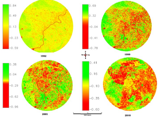
Figure III: Results of Land cover analysis
- Land use analysis :
Land-use analysis was performed using using the function i.maxlik (in GRASS) based on supervised classifier based on Gaussian maximum likelihood algorithm. Temporal land use is given in figure 4 and the statistics of category-wise land uses are for 5 time period is given in table IV. Urban category has increased from 13% (1992) to 33% (2010), which is about 253 times during the last two decades. Notable factor is that the Cultivation which is the major land use in the study region has increased to a small extent. Vegetation had decreased drastically over last two decades from 30% (1992) to about 6% (2010). The results of the overall accuracy for each classification map were 90% (1992), 90.33% (1999), 92.45% (2005) and 94.12% (2010). Kappa values were 0.84 (1992), 0.85 (1999), 0.9 (2005) and 0.91 (for 2010).
Table IV: Results of Land use analysis
| Class |
Urban % |
Vegetation % |
Water % |
Cultivation % |
| Years |
| 1992 |
13.58 |
30.94 |
1.52 |
53.95 |
| 1999 |
25.32 |
24.82 |
1.51 |
48.35 |
| 2005 |
28.16 |
10.09 |
1.12 |
60.62 |
| 2010 |
33.56 |
5.52 |
1.2 |
59.72 |
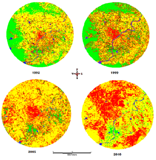
Figure 4: Results of Land use analysis
- Shannon’s Entropy :
Shannon entropy was calculated to understand the state of urbanization direction wise in the study region (either fragmented or clumped) and are given in Table V. The analysis show of sprawl in the North West, while significant growth was observed in North East, South East and South west but fragmented due to presence of cultivable land in these regions.
Table V: Results of Shannon’s entropy
|
NE |
NW |
SE |
SW |
| 1992 |
0.23 |
0.24 |
0.18 |
0.25 |
| 1999 |
0.39 |
0.41 |
0.34 |
0.36 |
| 2005 |
0.4 |
0.45 |
0.38 |
0.43 |
| 2010 |
0.43 |
0.7 |
0.42 |
0.47 |
| Reference value |
1.079 (Log(12)) |
- Landscape Metrics
Spatial metrics were computed using Fragstat(McGarigal and Marks, 1995)to understand the level of urban dynamics and are listed in table 2. FRAGSTAT requires details such as rows and columns that were obtained using g.region –p. Class properties file was created using the ascii text format as per the land use classes. The output of the land use for the gradients corresponding to 1km gradients was considered in 16 bit binary format and the spatial metrics were calculated direction wise for each gradient. Results of the analysis indicate of clumped growth at the center of the city and is in the verge of forming a single class patch. Compared to this, outskirts or peri-urban regions are fragmented or sprawl with different classes in the neighborhood. Metric results are quantitatively described next.
Proportion of Landscape (PLAND) and Largest Patch Index (LPI): PLAND is one of the metrics that’s calculated on the properties of the landscape. Pland approaches 0 when the land use class is rare in the landscape and the value will reach 100 when the entire landscape consists of a single patch type; intermediate values representing the degree of clumping or fragmentation. LPI = 0 when largest patch of the patch type becomes increasingly smaller as in the comparision of the landscape. LPI = 1 when when largest patch comprise 100% of the landscape (Wu et al., 2002, 2004). Results of the analysis of the PLAND metric is given in Figure 5a. Results reveal of phenomenal increase in urban area over the past decade . Outskirts neighborhood have large variability in land use classes but form single patches in 2010 especially in the north west and south west directions. The core area though clumped with urban class has lower PLAND due to the presence of water and cultivation categories as major land uses.
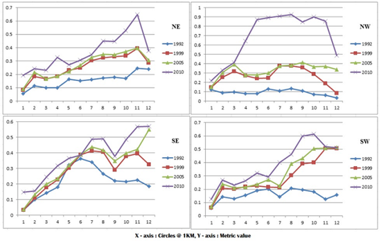
Figure 5a: Pland metric calculated for the study region
LPI (Figure 5b) indicates that the landcape is aggregating to form single patches in almost all directions and gradients. Fragmented outskirts are also now on the verge of forming a single patch, and core center is almost constant except in North east and south east directions as it has also water class which is comparatively a large patch.
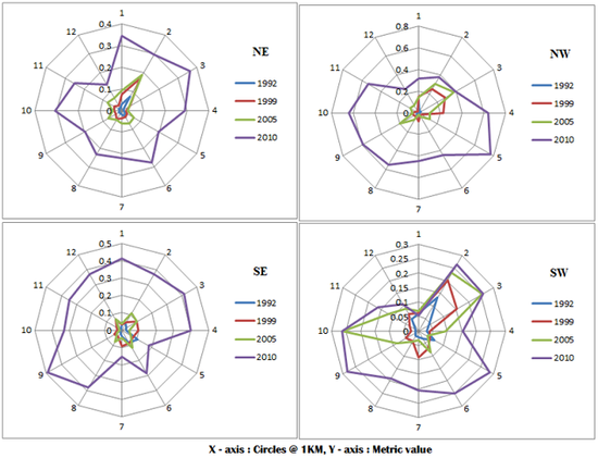
Figure 5b: Largest Patch Index
Number of Urban Patches (NP): NP reflects the extent of fragmentation (Baldwin et al., 2004, Turner et al., 1989) of a particular class in the landscape. Higher the value more the fragmentation, Lower values is indicative of clumped patch or patches forming a single class. The results (Figure 5c) show that center is in the verge of clumping especially accelerated in 2005 and 2010, while the outskirts remain fragmented and are highly fragmented during 2005 and 2010in North east, south east and south west directions. North west zone is losing its vegetation and cultivation class and this zone is highly fragmented in the outskirts during 2005 but is now in the verge of forming a single built up class.
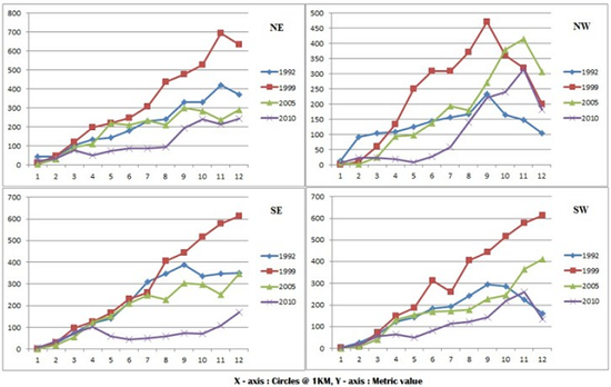
Figure 5c: Number of urban patches
Normalized Landscape Shape Index (NLSI): NLSI calculates the value based on particular class rather than landscape and is equal to zero when the landscape consists of single square or maximally compact almost square, its value increases when the patch types becomes increasingly disaggregated and is 1 when the patch type is maximally disaggregated. The results (Figure 5d) indicate that the urban area is almost clumped in all direction and all gradients especially in north east and west direction. It shows a small degree of fragmentation in the buffer regions in south west and south east direction. The core area is in the process of becoming maximally square in all directions.
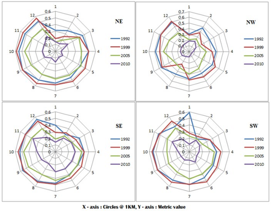
Figure 5d: NLSI index
Patch Density (PD): PD refers to number of patches per unit considered. This index is computed using a raster data with 4 neighbor algorithm. Patch density increases with a greater number of patches within a reference area. As seen before the fragmentation is large in the buffer regions and hence the patch density is high in the buffer region as compared to the core area. Patch density increased with number of patches increasing in mid-90’s further continued till 2005. During the years 2005- 2010 patch density considerably decreased as number of patches decreased and hence indicated the process of clumping. Figure 5e explains the patch density at patch level.
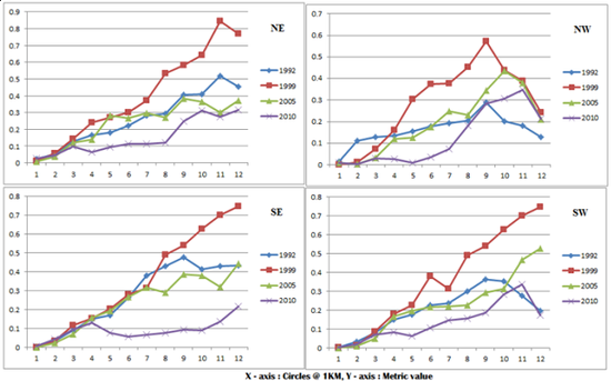
Figure 5e: Patch Density
Aggregation index (AI) and Clumpiness Index (Clumpy): AI and Clumpy are two measures of degree of fragmentation of the landscape. AI equals zero when the patches are maximally disaggregated and equals 100 when the patches are maximally aggregated into a single compact patch (Cushman et al., 2008, Bailey et al., 2007) and Clumpy equals 0 when the patches are distributed randomly, and approaches 1 when the patch type is maximally aggregated. Results of AI (Fig. 5f) are indicative of the clumpedness of the patches at the outskirts and buffer region and are fragmented in the central core. Clumpy (Figure 5g) also indicates the same as it is rather a proportion it also is indicative that the central core is fragmented, But in the process of clumping to form a single patch.
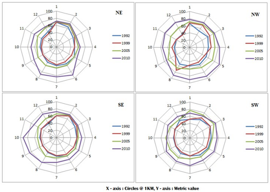
Figure 5f: Aggregation index
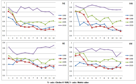
Figure 5g: Clumpiness index
Percentage of Like Adjacencies (PLADJ): PLADJ is the percentage of cell adjacencies involving the corresponding patch type that are like adjacencies. Cell adjacencies are tallied using the double-count method in which pixel order is preserved, at least for all internal adjacencies. equals 0 when the patch types are maximally disaggregated and there are no like adjacencies. PLADJ is 100 when all patch types are maximally and the landscape contains a border comprised entirely of the same class. The results (Figure 5h) indicate that the adjacencies are quite low in the core area as it has different patch types. Whereas high adjacencies are found in certain buffer zones of north west and south east directions. We can observe that the patches in 1998 and 2005 have disaggregation whereas in 2010 all patches are becoming aggregates.
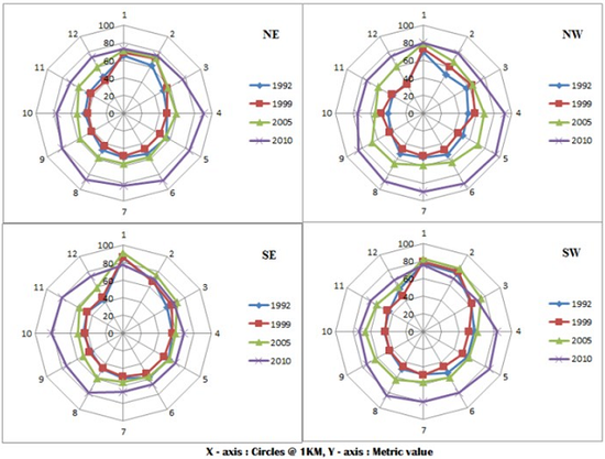
Figure 5h: Percentage of Land adjacency
Interspersion and Juxtaposition (IJI): Interspersion and Juxtaposition (Bailey et al., 2007) approaches 0 when the distribution of adjacencies among unique patch types becomes increasingly uneven. IJI is equal to 100 when all the patch types are equally adjacent to all other patch types. Analysis on the study region indicates (Figure 5i) that near the core the values are near zero indicating adjacencies are uneven whereas in the outskirts and buffer zones values are relatively higher indicating that they are relatively adjacent and clumped
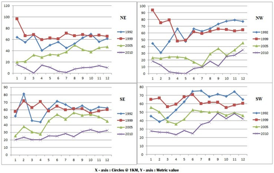
Figure 5i: IJI index
|
