|
DATA ANALYSIS
i. Preprocessing :
The remote sensing data corresponding to the study region were downloaded, geo-referenced, rectified and cropped pertaining to the administrative boundary with 5 km buffer. Landsat ETM+ bands of 2010 were corrected for the SLC-off by using image enhancement techniques, followed by nearest-neighbour interpolation.
ii. Land Cover Analysis :
Among different land cover indices, NDVI - Normalised Difference Vegetation Index was found appropriate NDVI was computed to understand the changes of land cover . NDVI is the most common measurement used for measuring vegetation cover. I t ranges from values -1 to +1. Very low values of NDVI (-0.1 and below) correspond to barren areas of rock, sand, or Urban builtup. Zero indicates the water cover. Moderate values represent low density of vegetation (0.1 to 0.3), while high values indicate vegetation (0.6 to 0.8).
iii. Land use analysis :
The method involves i) generation of False Colour Composite (FCC) of remote sensing data (bands – green, red and NIR). This helped in locating heterogeneous patches in the landscape ii) selection of training polygons (these correspond to heterogeneous patches in FCC) covering 15% of the study area and uniformly distributed over the entire study area, iii) loading these training polygons co-ordinates into pre-calibrated GPS, vi) collection of the corresponding attribute data (land use types) for these polygons from the field . GPS helped in locating respective training polygons in the field, iv) supplementing this information with Google Earth v) 60% of the training data has been used for classification, while the balance is used for validation or accuracy assessment.
Land use classification of Landsat satellite data was done using supervised pattern classifier - Gaussian maximum likelihood algorithm based on various classification decisions using probability and cost functions (Duda et al., 2000). Mean and covariance matrix are computed using estimate of maximum likelihood estimator. Land Use was computed using the temporal data through open source GIS: GRASS - Geographic Resource Analysis Support System (www.ces.iisc.ac.in/grass). Four major types of land use classes considered were built-up, vegetation, cultivation area (since major portion is under cultivation), and water body. 60% of the derived signatures (training polygons) were used for classification and the rest for validation. Recent remote sensing data (2010) was classified using the collected training samples. For earlier time data, training polygon along with attribute details were compiled from the historical published topographic maps, vegetation maps, revenue maps, etc. Median filter of 3X3 was applied to the classification-derived maps to reduce the effect of “salt & pepper” noise produced by the classification procedure. Statistical assessment of classifier performance based on the performance of spectral classification considering reference pixels is done which include computation of kappa (κ) statistics and overall (producer's and user's) accuracies.
iv. Density Gradient Analysis :
Further the classified image is then divided into four zones based on directions considering the central pixel (Central Business district) as Northwest (NW), Northeast (NE), Southwest (SW) and Southeast (SE) respectively. The growth of the urban areas was monitored in each zone separately through the computation of urban density for different periods.
v. Division of four zones to concentric circles and computation of spatial metrics :
Each zone was further divided into incrementing concentric circles of 1km radius from the center of the city. The built up density in each circle is monitored overtime using time series analysis. Landscape metrics were computed for each circle, zone wise using classified land use data at the landscape level with the help of FRAGSTATS (McGarigal and Marks, 1995). Table II details the spatial metrics considered for the analysis of urban dynamics at local levels.
vi. Computation of Shannon’s Entropy :
To determine whether the growth of urban areas was compact or divergent the Shannon’s entropy (Yeh and Liu, 2001; Li and Yeh, 2004; Lata et al., 2001; Sudhira et al., 2004; Pathan et al., 2007; Ramachandra et al.,2012) was computed direction wise for the study region. Shannon's entropy (Hn) given in equation 1, provide insights to the degree of spatial concentration or dispersion of geographical variables among ‘n’ concentric circles across Zones.
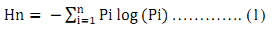
Where Pi is the proportion of the built-up in the ith concentric circle. As per Shannon’s Entropy, if the distribution is maximally concentrated the lowest value zero will be obtained. Conversely, if it evenly distribution the value would be closer to log n indicating dispersed growth or sprawl.
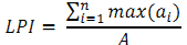
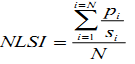
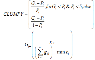
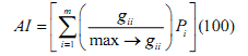
Table II: Landscape metrics calculated for the study region
|