|
Results & Discussion
1. Land use Land Cover analysis:
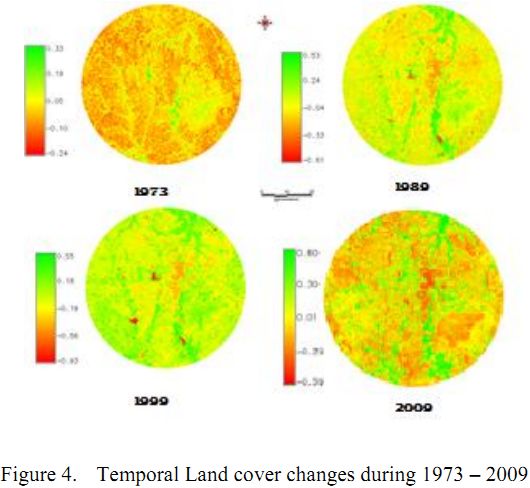
- Vegetation cover analysis: Vegetation cover of the study area assessed through NDVI (Figure 3), shows that area under vegetation has declined to 9.24% (2009) from 51.09% (1973). Temporal NDVI values are listed in Table III.
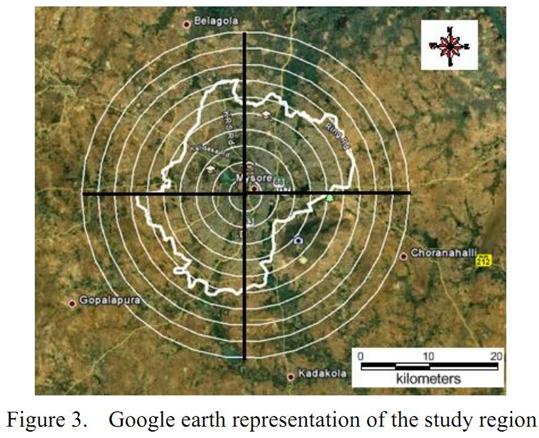
Figure 3. Google earth representation of the study region
Table III: Temporal Land cover details.
| Year |
Vegetation |
Non vegetation |
| % |
Ha |
% |
Ha |
| 1973 |
51.09 |
10255.554 |
48.81 |
9583.83 |
| 1989 |
57.58 |
34921.69 |
42.42 |
8529.8 |
| 1999 |
44.65 |
8978.2 |
55.35 |
11129.77 |
| 2009 |
09.24 |
1857.92 |
90.76 |
19625.41 |
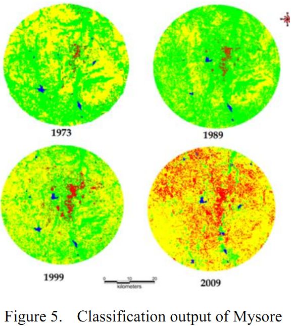
- Land use analysis: Land use assessed for the period 1973 to 2009 using Gaussian maximum likelihood classifier is listed Table IV and the same is depicted in figure 4. The overall accuracy of the classification ranges from 75% (1973), 79% (1989), 83% (1999) to 88% (2009) respectively. Kappa statistics and overall accuracy was calculated and is as listed in Table V. There has been a significant increase in built-up area during the last decade evident from 514% increase in urban area. Other category also had an enormous increase and covers 166 % of the land use. Consequent to these, vegetation cover has declined drastically during the past four decades. The water spread area has increased due to the commissioning of waste water treatment plants (ex. Vidyaranyapura, Rayankere, Kesare) during late 90’s and early 2000.

Figure 4: Temporal Land cover changes during 1973 – 2009
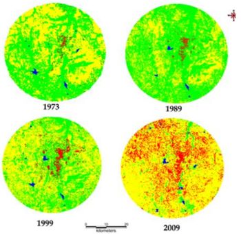
Figure 5:. Classification output of Mysore
Table IV: Temporal land use details for Mysore
| Land use |
Urban |
Vegetation |
Water |
Others |
| Year |
| 1973 |
222.93 |
10705.68 |
124.47 |
9054.99 |
| 1989 |
229.41 |
13242.51 |
78.75 |
6557.4 |
| 1999 |
730.8 |
8360.1 |
117.9 |
10899.2 |
| 2009 |
3757.489 |
1159.336 |
142.58 |
15050.5 |
| Total (Land in ha) 20108.91 |

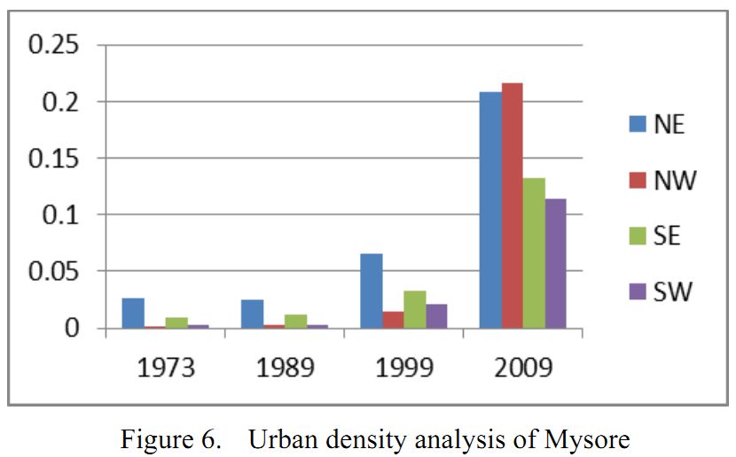
Figure 6: Urban density analysis of Mysore
2. Built up Density Gradient Analysis: Built up density was minimal and the value ranges from 0.026 (considering 3km buffer) to 0.036 (without considering 3km buffer) in the North east direction (in 1973). The federal government’s policy in 1990’s to develop tier 2 cities led to the increase in urban area. There was a sharp growth in the region in almost all direction from 1999 till 2009, maximum value reaching 0.216 in the NE direction (considering 3km buffer) and 0.42 (without considering the buffer). This can be attributed to development of this region with the IT & BT industry which were earlier confined to Bangalore.
3. Urban sprawl analysis: Shannon entropy computed using temporal data are listed in Table VI. Mysore is experiencing the sprawl in all directions as entropy values are closer to the threshold value (log (8) = 0.9). Lower entropy values of 0.007 (NW), 0.008 (SW) during 70’s shows an aggregated growth as most of urbanization were concentrated at city centre. However, the region experienced dispersed growth in 90’s reaching higher values of 0.452 (NE), 0.441 (NW) in 2009 during post 2000’s. The entropy computed for the city (without buffer regions) shows the sprawl phenomenon at outskirts. However, entropy values are comparatively lower when buffer region is considered. Shannon's entropy values of recent time confirms of minimal fragmented dispersed urban growth in the city. This also illustrates and establishes the influence of drivers of urbanization in various directions.
Table VI: Shannon Entropy Index
|
NE |
NW |
SE |
SW |
2009 |
0.452 |
0.441 |
0.346 |
0.305 |
1999 |
0.139 |
0.043 |
0.0711 |
0.050 |
1992 |
0.060 |
0.010 |
0.0292 |
0.007 |
1973 |
0.067 |
0.007 |
0.0265 |
0.008 |
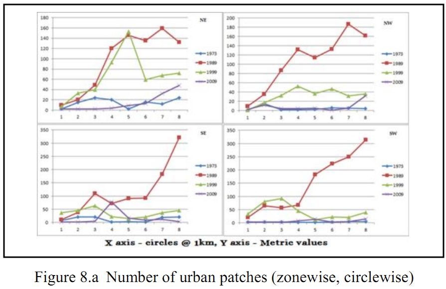
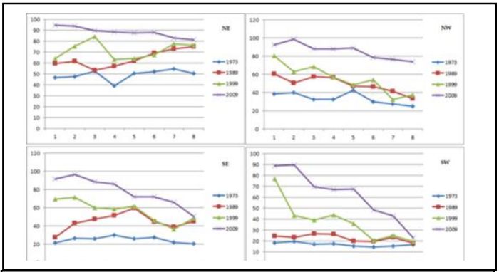
4. Spatial patterns of urbanisation: In order to understand the spatial pattern of urbanization, eleven landscape level metrics were computed zonewise for each circle. These metrics are discussed below: Number of Urban Patch (Np) is a landscape metric indicates the level of fragmentation and ranges from 0 (fragment) to 100 (clumpiness).
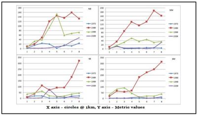
Figure 8a: Number of urban patches (zonewise, circlewise)
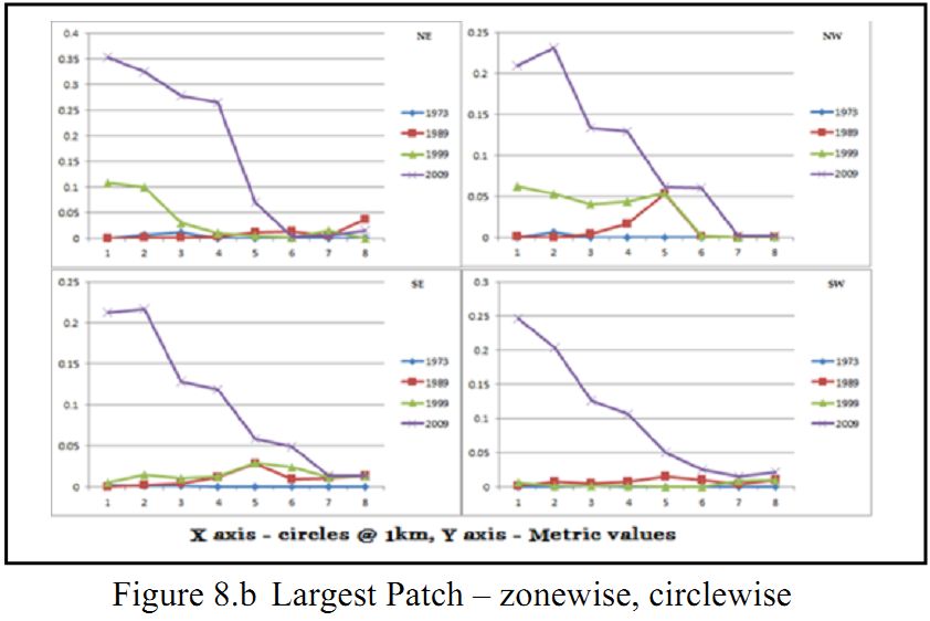
Figure 8a illustrates that the city is becoming clumped patch at the center, while outskirts are relatively fragmented. Clumped patches are more prominent in NE and NW directions and patchesis agglomerating to a single urban patch.Largest patch index (Fig 8b) highlights that the city’s landscape is fragmented in all direction (in 1973) due to heterogeneous landscapes, transformed a homogeneous single patch in 2009.The patch sizes given in figure 8c highlights that there were small urban patches in all directions (till 1999) and the increase in the LPI values implies increased urban patches during 2009 in the NE and SW. Higher values at the center indicates the aggregation at the center and in the verge of forming a single urban patch largest patches were found in NE and SW direction (2009).
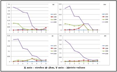
Fig 8b: Largest Patch – zonewise, circlewise
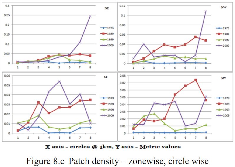
The patch density (Fig 8c) is calculated on a raster map, using a 4 neighbor algorithm. Patch density increases with a greater number of patches within a reference area. Patch density was higher in 1973 as the number of patches is higher in all directions and gradients due to presence of diverse land use, which remarkably increased post 1989 (NW) and subsequently reduced in 1999, indicating the sprawl in the region in in early 90’s and started to clump during 2009, which was even confirmed by number of patches.
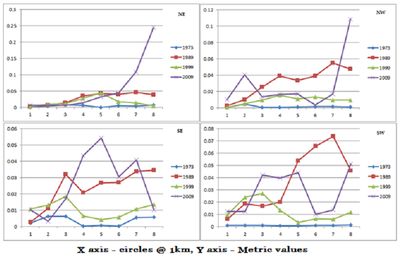
Fig 8c: Patch density – zonewise, circle wise
PAFRAC approaches 1 for shapes with very simple perimeters such as squares (indicating clumping of specific classes), and approaches 2 for shapes with highly convoluted, perimeters. PAFRAC requires patches to vary in size. Results (Fig 8d) indicate of dispersed development during 70’s and 80’s as PAFRAC highly convoluted. The value approaches 1 in 1990’s and 2000’s indicating aggregation leading to clumped region of urban land use.

Figure 8d: PAFRAC – zonewise, circle wise
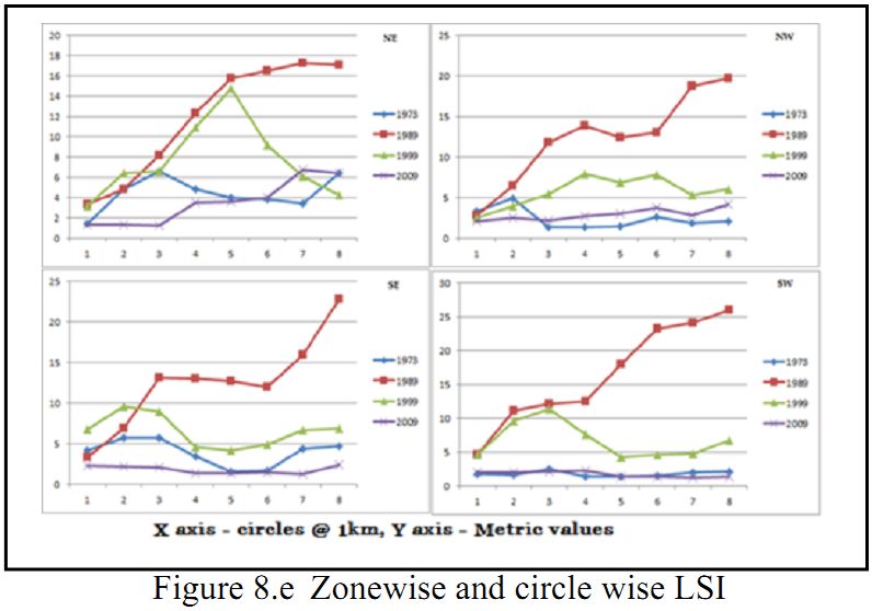
Landscape Shape Index (LSI): LSI equals to 1 when the landscape consists of a single square or maximally compact (i.e., almost square) patch of the corresponding type and LSI increases without limit as the patch type becomes more disaggregated. Results (Fig 8e) indicate that there were low LSI values in 1973 as there was minimal urban areas which were aggregated at the centre. Since 1990’s the city has been experiencing dispersed growth in all direction and circles, towards 2009 it shows a aggregating trend as the value reaches 1.
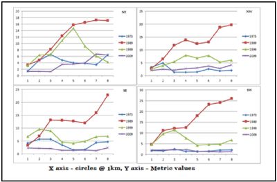
Figure 8e: Zonewise and circle wise LSI
Normalized Landscape Shape Index (NLSI): NLSI is 0 when the landscape consists of single square or maximally compact almost square, it increases as patch types becomes increasingly disaggregated and is 1 when the patch type is maximally disaggregated. Results (Fig 8f) indicates that the landscape had a highly fragmented urban class, which became further fragmented during 80’s and started clumping to form a single square in late 90’s especially in NE and NW direction in all circle and few inner circles in SE and SW directions, conforming with the other landscape metrics.

Figure 8f: Zone and circlewise NLSI
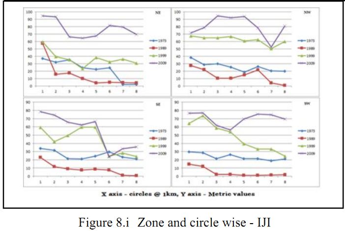
Clumpiness index equals 0 when the patches are distributed randomly, and approaches 1 when the patch type is maximally aggregated. Aggregation index equals 0 when the patches are maximally disaggregated and equals 100 when the patches are maximally aggregated into a single compact patch. IJI approaches 0 when distribution of adjacencies among unique patch types becomes increasingly uneven; is equal to 100 when all patch types are equally adjacent to all other patch types.
Clumpiness index, Aggregation index, Interspersion and Juxtaposition Index highlights that the center of the city is more compact in 2009 with more clumpiness and aggregation in NW and NE directions. In 1973 the results indicate that there were a small number of urban patches existing in all direction and in every circle and due to which disaggregation is more. Post 1999 and in 2009 we can observe large urban patches very close almost forming a single patch especially at the center and in NW direction in different gradients (Fig 8g, Fig 8h and Fig 8i).
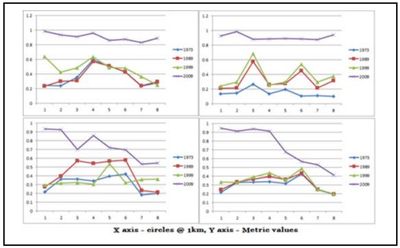
Figure 8g: Clumpiness – zonewise, circle wise

Figure 8h: Aggregation-zone and circle wise
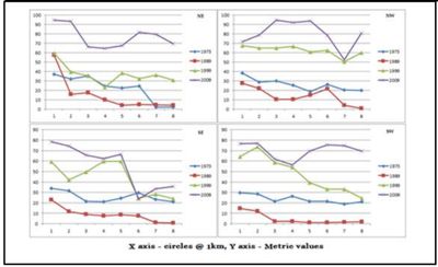
Figure 8i: Zone and circle wise -IJI
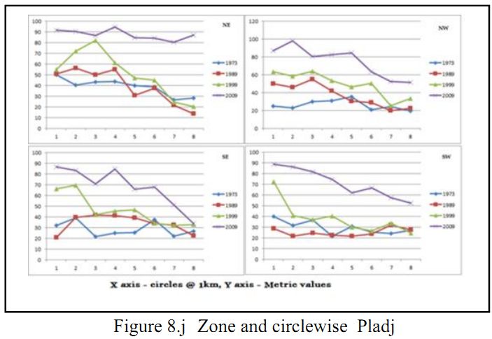
Percentage of Like Adjacencies (Pladj) is the percentage of cell adjacencies involving the corresponding patch type those are like adjacent. Cell adjacencies are tallied using the double-count method in which pixel order is preserved, at least for all internal adjacencies. This metrics also indicates the city center is getting more and more clumped with similar class (Urban) and outskirts are relatively sharing different internal adjacencies.
Patch cohesion index measures the physical connectedness of the corresponding patch type. This is sensitive to the aggregation of the focal class below the percolation threshold. Patch cohesion increases as the patch type becomes more clumped or aggregated in its distribution; hence, more physically connected. Above the percolation threshold, patch cohesion is not sensitive to patch configuration [18]. Figure 8k indicate of physical connectedness of the urban patch with the higher cohesion value (in 2009). Lower values in 1973 illustrate that the patches were rare in the landscape.
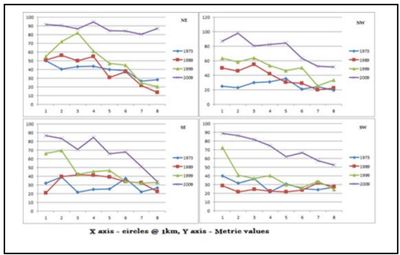
Figure 8j: Zone and circlewise Pladj

Figure 8k: Cohesion Index
|