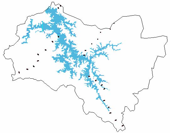
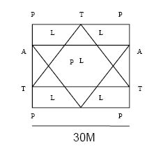
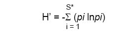
Materials and Methods

Land cover analysis was done to delineate the areas under vegetation and soil (non- vegetation). The land use analysis was carried out for the region to identify the use of land, emphasizing the functional role of the land in economic activities. Land use patterns reflects the characters of a society’s interaction with the physical environment, while land cover in its narrowest sense often designates only the vegetation cover extent on the Earth’s surface, as the spectral reflectance in green band (visible range of em spectrum) and near-infrared would represent the photosynthetically active vegetation. A cloud free IRS-1C satellite multi spectral imagery of LISS III sensors with spatial resolution of 23.5m was used for the analyses. Land cover analyses were done through computation of vegetation indices which could be Slope based or distance based (depending on the landscape type - hilly, arid, etc.). The Normalized Difference Vegetation Index (NDVI) was used to delineate vegetative from the non-vegetative features. High values in a vegetation index identify pixels covered by substantial proportions of healthy vegetation. Due to inverse relationship between vegetation brightness in the red (R) and near infrared (IR) region, a normalized difference ratioing strategy can be very effective. Once the extent of vegetation cover was determined, further analyses were done to classify image with field data. FCC image was generated by merging all 3 bands, which aided in identifying the heterogeneous patches for selection of training sites. Attribute information corresponding to these training sites were collected from field using Global Positioning System (GPS). In addition to this, GPS was used to map the tree species, which were sampled along 200 m transect with 20 x 20m quadrant. Gaussian maximum likelihood classifier was used to classify the data based on the attribute data collected from field. The statistical probability of a given pixel present in a specific land use category was calculated and each pixel in the data was categorized into the land use class it most closely resembled or the probability of occurrence.

SAMPLING STRATEGY FOR ANTS:
Sampling was done along four transects (Fig.2) moving away from the reservoir towards the end of the river basin. The undulating topography in the area resulted in non-uniform length of the transects that varied from 4 km to 32 km. Three sampling plots, 30 sq. m each, were located at every 4 km distance along the transects. These plots were placed in a mini-transect of 400 m at a 200 m interval, perpendicular to the main transect resulting in a total of 78 plots, distributed across moist deciduous forests, semievergreen, scrub jungles, acacia plantations, semievergreen forests, evergreen forests and pine plantations. At each of these plots the entire package of baits (described below) were laid for collecting ants. The catchment area being very small in the northern region (being very close to the dam), resulted in six (2x3) samples.

Fig 2: Sampling location for ants (Each sampling plot [30x30 sq m] is represented by a dot)

SAMPLING METHODS:
Ants live in different strata of the ecosystem as their nests vary from thick leaf litter, dead wood, modified nesting structures provided by plants, tree canopies and soil. In view of this ants cannot be collected by one technique and hence different methodologies of collection were employed. Ants were collected from each plot using bait traps, pitfall traps, leaf litter techniques and visual collections.

Terrestrial and arboreal baits were placed using 70% honey, tuna fish and fried coconut. Terrestrial baits (T) were placed on the ground (Fig 3) and the arboreal baits were tied to a tree at a height of 6 ft from the ground. A 10cm long cylindrical tube containing 90% ethyl alcohol with 3 drops of glycerin was used for a pitfall trap (P). A pit was dug with a mallet and the tubes were placed such that their mouth was flush with the ground. Five such pitfall traps were laid at every sample for a 24h period. The Burlese leaf litter technique was used in extracting ants from the leaf litter in four, 1x1m quadrants at each sub sample. The quadrants were placed in the four smaller quadrants (L), between the pitfall traps and baits in four directions. A visual collection was done for a period of an hour, which involved sweep net method, checking in barks, rotting logs and on leaves. From all traps insects were sorted and ants were separated for identification and preserved in 70% ethyl alcohol.

Fig 3: Sampling layout

ANALYSES:
As ant colonies show spatial clumping, counting the number of individuals of each captured species would be inappropriate. Hence the frequency of occurrence of each species in each habitat was determined and is termed as abundance. The Shannon’s diversity index is computed to determine ant diversity in habitats, which is a measure of the average degree of uncertainty in predicting to what species an individual chosen at random from a collection of S species and N individuals belongs. This diversity increases as the number of species increases and as the distribution of individuals among the species becomes even. It is given by,

where, H’ = average uncertainty per species in an infinite community made up of S* species with known proportional abundances p₁, p₂, p₃,…p_s; p_i = proportional abundance of i^th species (Ludwig and Reynolds, 1998).

Evenness across habitats was computed by the Pielou's evenness index, H'/logS, S being the number of species recorded over all the sites, wherein maximum values would be when all species are equally abundant.

Jaccards similarity index was used to analyze extent of similarity between habitats with respect to ant fauna. It is calculated as, O_ij = c/a + b – c; where, O_ij = overlap between habitats; c = no of species overlapping between i and j; a = no of species in habitat i; b = no of species in habitat j (Pramod, et al, 1997).

The maps of the study area were digitized using Mapinfo 5.0 (creation of vector layers). IDRISI was used to determine the NDVI index and also to arrive at a second level classification using a supervised classification approach - Maximum Likelihood Classifier (raster analyses). Geographic Resource Analysis Support System (GRASS) was used to build the 3-D image depicting high and low species richness of ants for the entire study area.