Study Area
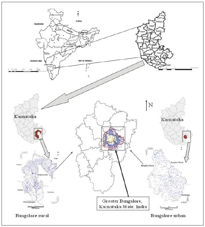
Greater Bangalore (77°37’19.54’’ E and 12°59’09.76’’ N) is the principal administrative, cultural, commercial, industrial, and knowledge capital of the state of Karnataka with an area of 741 square kilometres that lies between the latitudes 12°39’00’’ to 131°3’00’’N and longitude 77°22’00’’ to 77°52’00’’E. Bangalore city administrative jurisdiction was widened in 2006 by merging the existing area of Bangalore City spatial limits with eight neighboring Urban Local Bodies (ULBs) and 111 Villages of Bangalore Urban District (Sudhira, Ramachandra, & Bala Subramanya, 2007). Thus, Bangalore has grown spatially more than ten times since 1949 (69 square kilometres) and is a part of both the Bangalore urban and rural districts (Figure 1). Now, Bangalore is the fifth largest metropolis in India currently with a population of about seven million. The mean annual total rainfall is about 880 mm with about 60 rainy days a year over the last ten years. The summer temperature ranges from 18 °C – 38 °C, while the winter temperature ranges from 12 °C – 25 °C. Thus, Bangalore enjoys a salubrious climate all year round. Bangalore is located at an altitude of 920 metres above mean sea level, delineating four watersheds: Hebbal, Koramangala, Challaghatta and Vrishabhavathi watersheds. The undulating terrain in the region has facilitated creation of a large number of tanks for traditional uses such as irrigation, drinking, fishing, and washing. This led to the existence of hundreds of such water bodies in the past centuries of Bangalore. Even in early second half of the 20th century, in 1961, the number of lakes and tanks in the city stood at 262 (and the spatial extent of Bangalore was 112 square kilometres) and in 1985, the number of lakes and tanks was 81 (and the spatial extent of Bangalore was 161 square kilometres).
Data
Survey of India (SOI) toposheets of 1:50000 and 1:250000 scales were used to generate base layers of taluk boundaries, city boundary, drainage networks, and wetlands (Figure 1). Field data were collected with a handheld GPS. RS data used for the study are:
- Landsat MSS data of 1973 (79 m), Landsat TM of 1992 (30 m) [downloaded from http://glcf.umiacs.umd.edu/data/]
- MODIS 7 bands product of 2002 and 2007 (Band 1 and 2 = 250 m and Band 3 to 7 = 500m) [downloaded from http://edcdaac.usgs.gov/main.asp]
- IRS LISS-3 (23.5 m) data of 2006 procured from NRSA, Hyderabad, India
- Google Earth data (http://earth.google.com) served in pre and post classification process and validation of the results Landsat ETM+ (8 bands) of 2000
- SRTM (Shuttle Radar Topography Mission) elevation data of 90 m [downloaded from http://glcf.umiacs.umd.edu/data/]
To map wetlands, IR bands are appropriate as water entirely absorbs the energy in wavelengths (0.7–2.35 mm). Suitability of IR bands to extract water line was done successfully by Yamano, H., et al., (2006). The ability of five satellite sensor bands (IKONOS band 4, Terra ASTER bands 3 and 4, and Landsat ETM+ bands 4 and 5) were examined to extract the waterline at coral reef coasts using different wavelength regions (near infrared [NIR] and shortwave infrared [SWIR]) and different spatial resolutions (4, 15, and 30 m). After performing geo-referencing and normalization of images, density slicing was used to extract the waterline. Extracted waterline positions were compared with ground-level data of the island shorelines for eight transects using global positioning system (GPS).
Methods
The methods adopted in the analysis involved :
- Creation of base layers like district boundary, district with taluk and village boundaries, road network, drainage network, mapping of water bodies, etc. from the SOI toposheets of scale 1:250000 and 1:50000.
- Geo-referencing of acquired RS data to latitude-longitude coordinate system with Evrst 56 datum: Landsat bands, MODIS bands 1 and 2 (spatial resolution 250 m) and bands 3 to 7 (spatial resolution 500 m) were geo-corrected with the known ground control points (GCP’s). Re-projection from Sinusoidal to Polyconic with Evrst 1956 as the datum, followed by masking and cropping of the study area.
- Re-sampling using nearest neighborhood technique :
- NIR and MIR bands (bands 3 and 4) of Landsat 1973 data to 23.5 m.
- 3 IR bands of Landsat (band 4-NIR, 5-MIR and 7-MIR) of 1992 to 23.5 m.
- 4 IR MODIS bands 2 and 5 to 7 (MOD 09 product) to 250 m.
- Principal Component Analysis (PCA) : Principal components representing maximum variability of the original datasets were chosen based on eigen values with PCA (given in Appendix A) of MODIS bands 2, 5, 6 and 7.
- Principal components of MODIS data (250 m spatial resolution) were fused with IR Band (Band 3) of IRS LISS-3 MSS data (23.5 m spatial resolution) using RGB – HIS algorithm (Carper, Lillesand, & Kiefer, 1990) as discussed in Appendix B. The three principal components (PC1, PC2 and PC3) of the low resolution MODIS were transformed to IHS (I is intensity, H is hue, S is saturation). I was replaced with the IR band of LISS-3 (of spatial resolution 23.5 m). Then, the fused images were obtained by performing an inverse transformation of IHS back to the original RGB.
- K-means algorithm was used to partition the data samples in the feature space into disjoint subsets or clusters as discussed in Appendix C. The similarity between two data points was quantified using a distance measure that facilitates measurement of the clustering quality of a partition. Pixels were clustered into 4 groups – built-up, vegetation, wetlands and others (based on field knowledge) based on randomly chosen 4 seed pixels.
- The prior probability P(?k) for the kth class which is the proportion of the number of pixels in that class to the total number of pixels and the covariance matrix Sk were computed. A pixel was assigned to a particular class for which it has the maximum probability (details in Appendix D).
- Accuracy assessment of automatically extracted wetlands was done with field knowledge, visual interpretation and also referring Google Earth (http://earth.google.com).

HOME
