Data and Methods

Table 1 lists the data used in this study. Land use in the basin was analysed using remotely sensed data of the year 2014 acquired from Landsat 8 with resolution of 30 m. Collateral data includes base layers (boundary, drainage network, etc.) digitised from the Survey of India topographic maps of scale 1:50000 and 1:250000, Bhuvan, Google Earth and Western Ghats land use vector data of French Institute of Pondicherry, Puducherry (available at India Biodiversity Portal http://indiabiodiversity.org).  Daily Rainfall data starting obtained from Karnataka statistics Department, Bangalore and National Climatic Data Centre, NOAA between 1901 and 2012. Average monthly temperature data were obtained from Worldclim (http://worldclim.org), and monthly average rainfall data of WorldClim derived from NOAA was used to compare the interpolated data. Solar Irradiation data which is used to calculate the Potential Evapotranspiration was obtained from Food and Agriculture Organization. Watershed extent was delineated from topographic maps along with ASTER Digital Elevation Model (DEM) of 30 m resolution. Population data of 2001 and 2011 were obtained from Census of India data (http://censusindia.gov.in). District at a glance (http://des.kar.nic.in) publications were used to obtain data regarding livestock population and net agricultural area sown for different agricultural products. Crop calendar National Food Security Mission along with the water requirement during different growth phases were used to estimate the monthly water requirement of crops grown in the sub-catchment.

IV. Method

Method involved in understanding the dynamics of landscape on the hydrologic regime is as depicted in fig 6. The raw satellite data both optical and radar data were downloaded from the USGS [46] public domain. Ground control points were acquired from the Surevy of India topographic maps, field data, Google earth or Bhuvan to correct the remote sensing data.

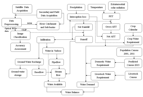
Optical images were checked for any inherent radiometric errors from the source. The digital elevation data from SRTM was used in order to delineate the catchment, watershed maps and stream network of the Lakshmanatirtha River, the DEM was supported in addition with the topo-sheets, Carto-DEM, ASTER to increase the precision in delineation. The catchment boundary and watershed maps were further used for the land use and hydrologic analysis. The Optical and Infrared bands of satellite data were used in order to characterize the land use of the catchment as well as the watersheds. To understand the information obtained from the satellite image, the optical and infrared bands such as Green, Red and Near-Infrared were combined together to prepare FCC i.e., false colour composite, to identify the heterogeneity in land use across the catchment. Training data were collected basin on ground knowledge and secondary data sources such as Bhuvan and Google earth, of which 70% of the training polygons were used to classify the image and the remaining 30% for accuracy assessment. Of the different soft classifiers, a very well proven algorithm i.e., Gaussian maximum likelihood algorithm [29, 30, 59] was used to classify the satellite image into various land use information as in table 2. Accuracy assessment and kappa analysis was carried out in order to check the accuracy and agreement of the classification result with the reference
Rainfall data for over 110 year from Statistics department of Karnataka and NOAA for the rain gauge stations inside and surrounding the catchment were interpolated in order to evaluate the rainfall spread across the catchment in different months. The interception loss was accounted as this is the water that is stored on the canopy of the vegetation and effectively doesn’t reach the earth surface, but escapes into atmosphere as evaporation. The net rainfall reaching the surface of the earth is derived as the difference between the gross rainfall and the interception in the watershed, and is used to effectively understand the hydrological variations in each of the watershed.

Runoff is the amount of water that flows in excess after the soil reaches its saturation condition and with reduction in the infiltration capacity of the soil under different land use criteria’s. Runoff Q is estimated empirically [26, 27] using equation 1, where C is the Coefficient of land use, A is the area under the land use and P is the Net Precipitation in mm. The Coefficient of Runoff for different land uses were considered is as in table 3.

Q = C*A*P             (1)
Of the percolated rain water, portion replenishes the ground water zone (saturated zone) and the balance is stored in the soil and sub soils up to the hypomorphic layer [60] referred to as vadose water. Portion of the vadose flows into the streams as pipe flow and portion of the ground water recharged, flows into the streams as base flow and the remaining recharges the aquifer. The ground water recharging capability of the basin is estimated using the Krishna Rao’s equation (equation 2), which is well suited for the study area.
GR = RC * (P – K) * A          (2)
where,
GR is the annual ground water recharge, RC is the recharge coefficient, K is the rainfall coefficient. Table 4 gives the details of the coefficients.

Table 2: Land Use Categorization

Fig. 6 : Method involved

Table 3: Runoff coefficients

Table 4: Ground water recharge coefficient and rainfall coefficient

The water in the vadose zone is taken as the difference of infiltration and ground water recharge. Partial of the recharged ground water goes to the stream as base flow BF, based on studies conducted earlier and field data, base flow BF into the stream is given by equation 3, the yield YS characteristics based on the geological criteria’s.

BF = GR * YS          (3)

The characteristics of the watershed such as runoff, vadose water and base flow contribute toward the water supply, whereas the demand in the watershed are due to evapotranspiration, agriculture and horticulture water requirement, domestic and livestock water requirement. The evapotranspiration is dependent upon characteristics such as temperature, solar radiation, and land uses in the basin, portion of the evaporation of the basin is taken care by the intercepted water. Evapotranspiration is calculated using equation 4.

AET = A*(PET - Interception)*Kc                   (4)

Where AET is the actual evapotranspiration, PET is the potential evapotranspiration and Kc is the evaporation coefficient based on the land use. PET (eq 5) is estimated using the Hargreaves equation which accounts the minimum and maximum temperatures and extra-terrestrial solar radiation. The evaporative coefficients for various land uses area as in table 5. The croplands and horticulture lands were not accounted for estimating the AET since the crop water requirements included the water requirement for each crop based on their growth phase.

PET = 0.0023 * (RA/λ) *  *                  (5)

where,                   
RA           = Extra-terrestrial radiation (MJ/m2/day)
Tmax     = Maximum temperature
Tmin      = Minimum temperature
λ              = latent heat of vaporization of water (2.501 MJ/kg)

Table 5: Evaporative Coefficients

The crop water demand (eq 6) for each crops were estimated by calculating the area under each crop, growth phase of each crop and water requirement based on different growth phases. Water requirement for livestock was estimated based on livestock type [61], number of animals under each category, water requirement per animal (table 6) and season. Livestock type and population were as per the publication - district at a glance.

Crop water Requirement (monthly) = Σ (Area under each crop * Crop water required under each crop)         (6)

P2013 = P2011 * (1 + 0.2 * r2001-2011)        (7)

Table 6: Livestock water requirement as litre/animal

Domestic demand, similar to live stock, was estimated as product of population for the year 2013 under each basin and water requirements based on season (table 7). Population for the year 2013 P2013 was estimated by using the growth rate between 2001 and 2011 r2001-2011, and population of the year 2011 P2011, to estimate the population rate of interest method (equation 7) was used

Table 7: Domestic water requirement as lpcd

Both the demand and supply for every month were analysed to assess the hydrological status of the basin in order to cater the needs of the environment, agricultural, domestic and livestock needs. If the supply is lesser than that of demand, the catchment is said to be in high water stress condition, else the water in the watershed catering the current needs there by in other words maintaining the environmental flow of the catchment. For more precision, the needs such as industrial, hydro-power, fish and other water requirement along with characteristics such as timing of flow, quality, and quantity can be supplemented.