Materials and Methods

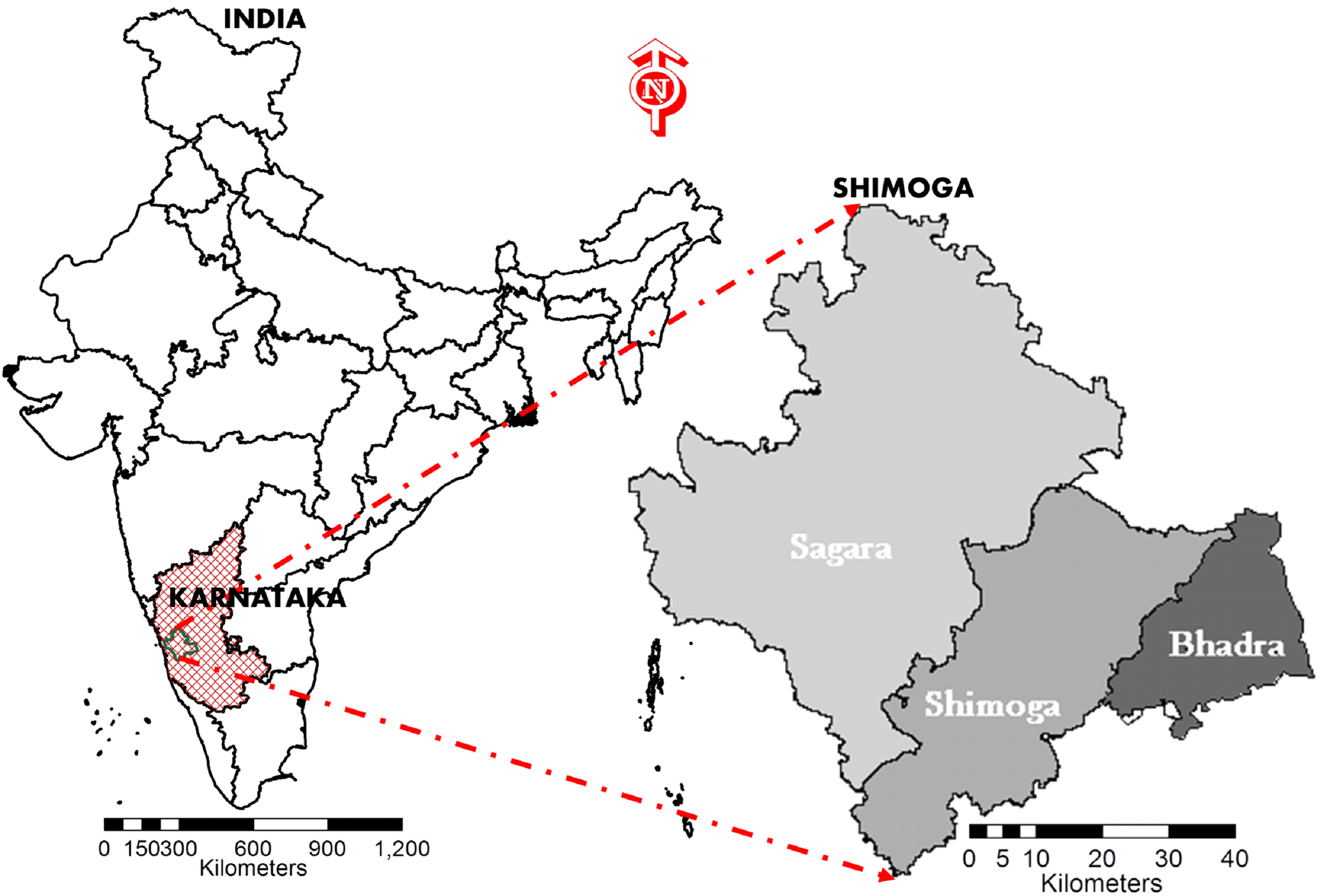
Shimoga or “Shivamogga” or "Shiva-Mukha" district lies between 13⁰ 27’ to 14⁰ 39’ N latitude and 74⁰ 37’ to 75⁰ 53’ E longitude, with a spatial extent of 8,495 km² spread across 1530 villages. Agriculture and animal husbandry are the major contributors to the economy of Shimoga district. The climate is tropical wet and dry and temperature ranges between 37 ^oC (Max) to 23.2 ^oC (Min). The district receives an average rainfall of 1813 mm. Shimoga district is divided into 2 sub-divisions (Sagara and Shimoga), 7 taluks (Shimoga, Bhadravathi, Thirthahalli), and 3 forest divisions (Sagara, Shimoga, Bhadra) (Fig. 1). As per the 2011 census, the population of the district is 17,55,512 with a density of 207 persons per sq.km. Shimoga is an ideal destination for tourism across the seasons due to dense forests, hills, splendidly diverging waterfalls, and religious places with diverse cultures. The region is home to rich diverse flora such as Alangium salviifolium, Artocarpus heterophyllus, Artocarpus hirsutus, Holigarna grahamii, Holigarna nigra, Mangifera indica, Caryota urens, Canarium strictum, Garcinia gummi-gutta, Grewia tiliifolia, Hopea ponga, Hopea Jacobi, Cinnamomum malabatrum, Saraca asoca, Lagerstroemia microcarpa, Memecylon talbotianum, Ficus nervosa, Knema attenuate, Myristica malabarica, Syzygium travancoricum, Santalum album etc. The faunal species include Bos gaurus, Macaca Silenus, Panthera pardus, Panthera tigris, Rusa unicolor, Sus scrofa, Indirana beddomii, Nyctibatrachus beddomii, Philautus leucorhinus, Ramanella montana, Apus affinis, Chalcophaps indica, Vanellus indicus, Halisatur indicus, Pavo cristatus, Ocyceros griseus, Dicrurus pradiseus, Catla catla, Garra mullya, Labeo rohita, Puntius carnaticus, Schistura nagodiensis, Schistura Sharavathyensis, Geckoella albofasciatus, Kaestlea beddomii, Naja naja, Trimeresurus malabaricus, Varanus bengalensis etc. Protected Areas such as the Sharavathy Wildlife Sanctuary, Someshwara Wildlife Sanctuary Shettihalli Wildlife Sanctuary, and Gudavi Bird Sanctuary are with diverse flora and faunal species.

2.2 Data

Multiresolution spatial data acquired from Landsat and IRS multispectral sensors for the period 1973 to 2018, listed in Table 1, were downloaded from the respective web portals. These data are resampled to 30 m to maintain common resolution across the datasets. The Landsat satellite 1972 images have a spatial resolution of 57.5 m x 57.5 m (nominal resolution) was resampled to 30 m comparable to other data which are 30×30 m (nominal resolution) as per the standard protocol reported earlier (Pohl, 1996; Gupta et al. 2000; Kumar et al. 2010; West et al. 2014). Radiometric corrections were implemented by transforming raw digital numbers (DN) to radiance or reflectance, considering band-specific additive or multiplicative rescaling factor from metadata with the quantized and calibrated standard product pixel values (DN). The Survey of India (SOI) topographic maps were used to generate base layers of administrative boundaries, ground control points (GCP’s), etc. Ground control points to register and geo-correct remote sensing data were also collected using handheld pre-calibrated GPS (Global Positioning System). Collateral data used for geo-rectification and classification include geo-referenced topographic maps of the Survey of India, historical vegetation maps (from Karnataka Forest Department, Shimoga division), Vegetation map of South India (French Institute, Pondicherry), Annual Progress reports of the Karnataka Forest Department and other government agencies. In addition to these, the location-specific field data is being collected during the past three decades in the central Western Ghats as part of the ongoing ecological research pertaining to vegetation, monitoring of riverine ecosystems, etc. This aided in compiling training polygons (with attribute information) for remote sensing data classification and accuracy assessment.

Table 1 Data used in the analyses of landscape dynamics

2.3 Method

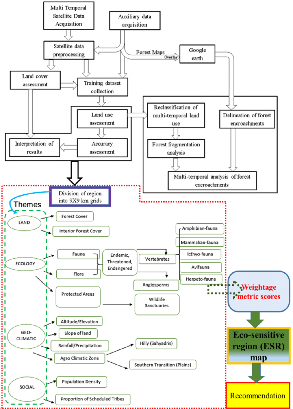
The spatio-temporal LULC changes were studied and ecological sensitive villages are demarcated as outlined in Fig. 2. The analyses have been carried out in three stages namely (i) LULC change estimation, (ii) fragmentation analysis with casual factors estimation, and (iii) prioritization of region based on ecological sensitiveness.

2.3.1 Quantification of Land Use Land Cover dynamics

Spatiotemporal analyses involved determining the land use and land cover changes using geo-registered temporal remote sensing data. The monitoring of LC involves the computation of vegetation indices, which enables assessing the extent of vegetation cover over non-vegetation. Land cover was determined through the computation of NDVI (Normalized Difference Vegetation Index) as per equation 1 (Table 2), based on the spectral difference of vegetation absorbance in the red during photosynthesis and reflectance in the near-infrared wavelength of the spectrum. Among all techniques of vegetation mapping, NDVI is most widely accepted (Zhang and Zhang 2007; Jensen and Toll 1982; Nelson 1983) technique with a capability to bring out changes in LC and extract changes through automated change detection techniques from temporal remote sensing data (Roy et al. 2002; Ramachandra et al. 2014).

LU analyses involved i) geo-rectification of remote sensing data; (ii) developing False Color Composite (FCC) using 3 bands (bands – green, red and NIR) of remote sensing data, which aided in locating heterogeneous patches; iii) digitization of training polygons (corresponding to heterogeneous patches in FCC) uniformly distributed over the entire study area, covering 15% of the study area; and, iv) collecting the attribute data (land use types) of these training polygons from the field using pre-calibrated GPS; iv) collecting additional information from the latest spatial data available at virtual spatial portal - Google Earth and Bhuvan; and v) using 60% of the training data for classification, and the balance during the post-classification for validation or accuracy assessment.

LU categories were derived from the remote sensing data, based on the Gaussian maximum likelihood algorithm using the supervised classification technique. This approach preserves the basic LU characteristics using a number of well-distributed training pixels. Gaussian Maximum Likelihood algorithm is an efficient method among supervised classification techniques based on training data or “ground truth” information. Geographical Analysis Support System (GRASS) GIS, a free and opensource software accessible at http://wgbis.ces.iisc.ernet.in/grass/index.php, with the robust processing capability of both vector and raster files. Accuracy assessments help in assessing the quality of the information derived from remotely sensed data by a set of reference pixels. These test samples are then used to create an error matrix (also referred as confusion matrix) kappa (κ) statistics and producer's and user's accuracies to assess the classification accuracies. Kappa is an accuracy statistic that permits us to compare two or more matrices and weighs cells in error matrix according to the magnitude of misclassification. The accuracy of pre-2002 images was assessed based on the collateral data (geo-referenced the survey of India toposheets of 1:50000, vegetation map of South India of 1:250000, published reports and the field data collected during the past three decades in the central Western Ghats pertaining to vegetation sampling, monitoring of riverine ecosystems, etc.). Availability virtual earth portals (such as Bhuvan, Google Earth) during post-2002 also helped in classification and accuracy assessment.

Table 2 Equations used for the analysis

2.3.2 Fragmentation analysis

Fragmentation of forests is assessed using spatial metrics such as Number of Patches (NP), Patch Density (PD), Total Edge (TE), Edge Density (ED), Landscape Shape Index (LSI) and Aggregation Index (AI) using Fragstats free software (Equation 2-7, Table 2). These metrics were calculated with a moving window of 5×5 (Neel et al. 2004; McGarigal et al. 2005; Ramachandra et al. 2012b; Bharath et al. 2017) that aid in assessing the neighborhood alterations in its spatial quantity.

Fragmentation through Pf and Pff: Further to understand the level of degradation /deforestation ‘Pf and Pff’ were computed to quantify the type of forest fragmentation as shown in Equation 8 and 9, Table 2 (Ritters et al. 2000; Ramachandra and Kumar 2011; Ramachandra et al. 2016a). The result is stored at the location of the center pixel. Based on the knowledge of Pf and Pff, six fragmentation categories were derived as Interior (Pf= 1.0); patch (Pf< 0.4); transitional (0.4 < Pf< 0.6); edge (Pf> 0.6 and Pf– Pff> 0); perforated (Pf> 0.6 and Pf – Pff < 0), and non-forest.

2.3.3 Assessing the causal factors of forest degradation

Forests in Shimoga are administered through three divisions by the Karnataka Forest Department. The geo-registered administrative boundaries of forests in respective divisions were obtained from the Karnataka state forest department. These layers were overlaid on higher spatial resolution spatial data (Google Earth) to assess the forest changes within the respective boundaries. These regions are overlaid on classified land use layer to ascertain the type of land conversions (for example forest to agriculture/plantations).

2.3.4 Identification of Ecologically Sensitive Regions (ESR)

The study area is divided into 5’×5’ equal area grids (74) to account for the changes at microscale for assessing ecological sensitiveness. The data of various themes were compiled from field surveys, published literature, unpublished datasets, etc. A detailed database is created considering various themes covering geo-climatic, ecological, and social variables (Table 3). The weightage metric score is computed using equation 10 (Table 2 and Table 3) to reflect the priorities/significance associated with the respective theme. Developing a weightage metric score requires knowledge from a wide array of disciplines (Termorshuizen and Opdam 2009), planning should acknowledge and actively integrate present and future landscape needs. In particular, the weightages, which is based on an individual proxy and draws extensively on GIS techniques, stands out as the most effective method. The aggregated weightage (Equation 10, Table 3) for each grid (region) is generated and grouped based on mean and standard deviation to determine the various levels of sensitivities. The final ESR map will aid in decision making towards the conservation of ecologically sensitive regions through effective natural resource planning (Ramachandra et al. 2017).

Table 3 Variables considered for ESR mapping