1.1 Introduction
An ecosystem is a biotic and functional system/unit, which is able to sustain life and includes all biological and non-biological variables in that unit. Ecosystems are studied with an objective to understand them in their entirety, giving more insight than the sum of knowledge about its parts relative to the structure, metabolism, and bio-geochemistry of the landscape. Models of ecological processes are developed to further the understanding of the dynamics, structures, and functional interrelations of ecosystems. This would help preserve certain characteristics of an ecosystem (e.g., biodiversity, ecology, hydrology, etc.), with appropriate land-use strategies. They can be used to test which of the land-use strategies examined is most ecologically sound. Land-use strategies derived from ecological modelling provide a way of combining land use and ecosystem conservation. Ecosystem modelling requires management of geographically referenced spatial information detailing complex interactions between climatic, topographic, hydrologic, pedological, and ecological processes. Ecological models are formal expressions of the essential elements of the ecosystem in mathematical terms, which would help understand complex interactions in time and space better. Thus, ecological model simulations will aid as a sort of substitute experiment. However, for translation into conservation practice, it is essential that they are also accepted by land users and decision-makers.
Ecological modelling combines mathematical modelling, systems analysis, and computer techniques with ecology and management of the environment and its natural resources (Jorgensen 2003). It requires comprehensive knowledge on the functioning of ecosystem. It is extremely important to find a balanced complexity considering the available data, the ecosystem, and the focal problem (Jorgensen 1999; Jorgensen and Bendoricchio 2001). The nature of the ecological systems encompasses large spatial and temporal scales, multi-component, multi-scale, multi-disciplinary, multivariate, non-linear and complex systems (Wainwright and Mulligan 2004). A good model is typically based on the understanding of the ecosystem, availability of quality data, and the type of questions posed (or problems for which the model is developed) as illustrated in Figure 1.1. Modelling requires reasoning about the aims and intentions of the problem, and the most effective means of applying the decisions about these to model construction, while being economical at the same time with the available resources.
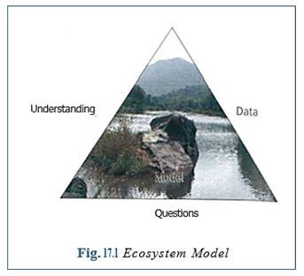 Figure 1.1. Ecosystem Model
Ecological investigations in the field can only be carried out in a few places and over short periods of time. Ecological models combine these detailed information in a logical manner and enable conclusions to be drawn for larger areas and longer periods. In addition, models can assist the process of decision-making, even if the information available is limited. The models can be divided into two classes, namely, general and specific. General models explain fundamental mechanisms to convey a basic understanding of certain functional interrelations. On the other hand, specific models focus on certain species, communities of species, or particular ecosystems
Ecological models can be further classified into static, dynamic, deterministic, and stochastic models. Some approaches to understand the dynamics of the ecosystem are:
- Empiricith: Complete picture of a system based on compiled data. Here attempts are made to integrate and assemble through compiled bits of information.
- Comparative: A few structural and functional components are compared for a range of ecosystem types.
- Experimental: Manipulation of an entire ecosystem is used to identify and elucidate on mechanisms.
- Modelling: Simulation studies.
The initial focus of modelling is the definition of the problem which is bound by the constituents of space, time, and subsystems. The bounding of the problem in space and time is more explicit than the identification of the subsystems to be incorporated in the model. Information, knowledge, data, and sometimes assumptions and estimates, are logically combined within the models. Elements of modelling in its mathematical formulations are listed in Table 1.1.
| Elements |
Description of Functional Aspects |
| Forcing functions or external variables |
These are functions or variables of an external nature, which influence the state of the ecosystem. The model is used to predict the change in the ecosystem when forcing functions are varied with time. The forcing function is often referred to as control function |
| State variables |
This describes the state of the ecosystem. Selection of state variables is crucial to the model structure. |
| Mathematical equations |
Describe the relationships between the forcing functions and state variables. Equations are used to represent biological, physical, and chemical processes. However, the number of details needed or desired to be included in the model may vary from case to case due to difference in complexity of the system and/or the problem |
| Parameters |
These are co-efficients in the mathematical representation of processes and are considered constant for a specific ecosystem or part of an ecosystem. But, the application of parameters as constants is unrealistic due to many feedbacks in real ecosystems. Flexibility and adaptability of ecosystems are inconsistent with the application of constant parameters in the models. In this context, varying parameters according to ecological principles is the solution |
| Universal constants |
Gas constants or atomic weights are also used in models |
Table 1.1 Elements of modelling
Significant steps in the modelling procedure are verification, calibration, and validation.
- Verification is to test the internal logic of the model, and, to some extent, a subjective assessment of the behaviour of the model before the calibration phase. Sensitivity analysis follows the verification process to obtain an overview of the most sensitive components of the model.
- Calibration is to find the best accordance between computed and observed data through variation of selected parameters.
- Validation consists of an objective test to find out how well the model output fits the data. It could be structural (qualitative) or a predictive (quantitative) validity. A model is structurally valid if the model structure represents reasonably and accurately the cause-effect relationship of the real system. A model exhibits predictive validity if its predictions of the system behaviour are reasonably in accordance with observations of the real system.
The success of calibration and validation is closely linked with the quality and quantity of the data. Modelling strategy is summarized in Figure 1.2.
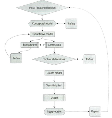 Figure 1.2. Modelling Strategy
Steps involved in modelling (Jackson, Trebitz, and Cottingham 2000) are as follows.
• A proper understanding of the problem is prerequisite before stepping into modelling
• Objectives must be very clear and properly defined (without ambiguity)
• A flow chart of the system
• Formulation of equations
• Assumptions required by equations
• Implement equations in computer code
• Verify equations
- unit checking
- compare numerical with analytical solutions
- compare with alternative coding
- study code and equations
• Analyse
- validation: one model
- model selection: > 1 model
- steady state, composition, stability
- sensitivity, error analysis
- risk assessment
- model experiments
• Draw conclusions, make predictions.
• Evaluate model relative to objectives
Ecological models are techniques that simulate the ecological systems and processes, which are tools to understand ecological processes and complexities of the ecosystem. Origin of ecological modelling dates back to the 1920s with Lotka-Volterra models of population dynamics and Streeter-Phelps model of dissolved oxygen in stream, but their comprehensive usage in environmental management began only during the 1970s. Abstraction and interpretation form two important procedures to link the model with the prototype or reality. Since many system properties are not represented in the model, hence it is up to the modeller, as to what parameters he requires (abstraction from the reality). Similarly, some model properties cannot be found in real systems, xvherein interpretation ability of the modeller gains in importance. A good model is typically based on the understanding of the ecosystem, availability of quality data, and the type of questions posed (or a problem for which the model is developed). Models have been used as a tool to solve problems, which are, in other words, simplified version of reality. Ecological models are also of similar kind, wherein management or scientific problems, species distribution, population dynamics, or for that matter, any ecological issue is addressed with certain characteristic features as input, and realized through appropriate mathematical operations and functions. Models can be used both as management tool and scientific tool. With sound ecological knowledge, it is possible to extract features of the ecosystem that are involved in the pollution problem udder consideration, to form the basis of the ecological model.
The first analytical ecological models appeared in the 1950s. With the advent of computers, many relationships between ecological factors and system processes have been derived. Models are classified into two groups:
(a) traditional process-based modelling, which are now actively combined with GIS spatial modelling; and
(b) ecological modelling, based on the information hierarchical approach presented as a system analytical model.
The application of models in ecology is pervasive, to understand the function of a complex system, such as an ecosystem. Over the last decade, ecological modelling has progressed emphatically due to improved understanding of quantitative relationships in the ecosystem between ecological properties and environmental factors (Jorgensen 2003) and the technical capabilities for handling of complex mathematical equations. Progress in ecological modelling and the great diversity of natural systems have given rise to a wide variety of models.
Currently, there is a large and continuously growing quantity of different mathematical models dealing with various ecological and environmental systems. On the whole, all approaches in ecological modelling can be divided into two types: empirical and analytical (there are many intermediate methods that are a combination of these two). Empirical approaches do not pursue the goal of the elucidation of the structural/functional (physical, biochemical, or other) organization of the system and use different methods of mathematical statistics. In contrast, analytical approaches pursue this goal and analyse the organization as such. Modelling plays a key role in the progression and consolidation of knowledge in ecology, i.e., from relatively knowledge-oriented but with poor data, giving scope to heuristic models to knowledge- and data-rich cases to build complex predictive models.
Ecological models are designed to simulate and predict fundamental ecological processes with reference to spatial and temporal landscape patterns on the watershed scale. Landscapes are heterogeneous (group of interacting ecosystems) and differ structurally in the distribution of species, energy, and materials among the patches, corridors and matrix present. Consequently, landscapes differ functionally in the flow of species, energy and materials among these structural landscape elements. Thus, structural and functional aspects, along with the changes in the landscape (spatio-temporal) forms a core theme of landscape ecological analysis. It hypothesizes that spatial arrangement of ecosystems, habitats, or communities has significant ecological implications. The characterization of landscape (shape, size, position, and other constituents) is done using remote sensing, in conjugation with Geographical Information System, and Global Positioning System. The interactions and flow of species (animals or plants), energy, water, and mineral nutrient among landscape elements emphasize the focal points within a landscape. Such focal points require special management practices to maintain connectivity, width of the corridors, and to avoid breaks and further enhancement of the process. Understanding landscape dynamics has become an important component of ecosystem management, as it quantifies the relationship of structural and functional components at various scales. Forest conservation, restoration, and management require the knowledge of ecological conditions and landscape dynamics.
Spatial and temporal patterns of landscape are replicated across a grid of cells that compose the rasterized landscape. Different habitats and land use types translate into different parameter sets to be fed into the ecological model. Cells are linked by horizontal fluxes of material and information, driven generally by the hydrologic flows. This approach provides additional flexibility in scaling up and down over a range of spatial resolutions, and is essential to track the land-use change patterns generated by the anthropogenic pressures. Large watersheds are composed of multiple smaller catchments. Each of these contains a heterogeneous collection of land uses, which vary in composition and spatial pattern (structure), and thus differ in functions such as nutrient retention, hydrological process, etc. Two problems arise from this heterogeneity that present major challenges to both research and management. First, variation in structure and function inevitably prevents true replication in intensive field studies that attempt to relate landscape function to landscape structure. Second, variation among land uses within watersheds makes it difficult to directly extrapolate among spatial scales. Even though watershed can be broken down hierarchically into smaller catchments based on topography, "scaling up" from intensive catchment studies is not a linear additive process because of differences among catchments and interactions between adjacent land uses. Management of water quality over large drainage basins needs to address both problems with innovative methods synthesizing data from intensive experimental studies on a few watersheds, and then extrapolating important generalizations to larger drainages using modelling techniques.
1.2. Deforestation Analysis through Metrics of Pattern Change
Landscape modification and loss of habitat continue to be the major factors impacting biodiversitY. These challenges are occurring at a time tivlleln there is a growing appreciation of the dynamic processes at the landscape scale (Naveh and Lieberman 1984; Zonneveld and Forman 1990). The influence of landscape pattern on the dynamics of species population has become a fundamental issue in resource management. The loss of forests worldwide may have contributed to global warming and escalating species extinctions (McNeely, Miller, Reid et al. 1990; Trani 19%). Ecological consequences can differ depending on the pattern imposed on a landscape. Pattern change is often accompanied by changes in the composition and persistence of species dependent on that habitat.
Deforestation can result in the decline of large, wide-ranging species (Pelton 1986); and in the loss of other specialized species (Rosenberg and Raphael 1986). The absence of forested corridors within a landscape hinders movement for some species (Harris 1988), while the altered size and shape of forest patches influences both biotic and abiotic processes (Van Dorp and Opdam 1987). Deforestation can also change the distribution and availability of spatial resources, influencing the components of forest connectivity (Noss and Harris 1986) and edge characteristics (Yahner 1988) that are important for the persistence of other species.
The landscape context of management planning makes examining potential methods for evaluating deforestation important. Environmental monitoring, dictated by stringent laws, requires using landscape analyses for projecting future landscape conditions. Using Geographic Information System technology, it is possible to model landscape deforestation and examine the effect on several measures of landscape pattern. Cartographic models generalize spatial relationships using the location and configuration of landscape elements. The development of spatial analyses for quantifying how deforestation influences pattern may prove useful for resource managers. The spatial heterogeneity metrics expresses the complexity and variability among the la,nd classes occurring on a landscape. The Shannon, Simpson, and binary comparison matrix indices are based on the number and proportions of land classes. Dominance measures the extent to which one or more classes dominate the landscape, while evenness refers to how abundance is distributed among those classes. The arrangement of land classes is reflected by the spatial diversity, number of different classes, and interspersion metrics. The fragmentation category of pattern metrics describes, in some manner, the amount of forest cover on a landscape. This group includes several patch metrics that reflect the number (patch density, number of forest patches), size (mean patch size), or degree of isolation (interpatch distance) of forest patches on a landscape. Fragmentation index ll (the average distance to non-forested areas) and per cent interior forest (the amount of forest area remaining after removing a buffer from the edge of each forested tract) are influenced by the distribution and amount of forest cover. Fragmentation index I reflects the number of distinct landscape regions on a map relative to the total number of map pixels.
The edge metrics characterize areas where two different land classes come together. Total forest edge refers to the length of edge that exists at the interface between a forest and other land classes. The convexity index is a perimeter-to-area ratio that describes the amount of edge per unit area of forest. The pattern and compactness indices compare the amount of forest edge and area in a landscape to that of a circle, and are considered shape metrics. The connectivity metrics describe the spatial connectedness of a landscape. Patchiness expresses the lack of connectedness, while the connectivity index detects the connections among forest patches. Forest contiguity assesses the unbroken adjacency of a forested landscape. The spatial integrity metric describes the spatial balance of a landscape by contrasting the number of forest openings with the number of existing patches. Pattern metrics listed in Table 1.2 helps analyse aspects of spatial heterogeneity, fragmentation, edge characteristics, and connectivity. Selection was based on their utility for landscape assessment and their potential relevance to biodiversity.
| Landscape Pattern Expression |
References |
| Spatial heterogeneity |
| Shannon index |
Shannon and Weaver (1963) |
| Dominance index |
O'Neil et al. 1988 |
| Different classes/number of categories |
Murphy (1985) |
| Simpson index |
Simpson (1949), Pielou (1977) |
| Landscape evenness |
Romme (1997) |
| Interspersion |
Eastman (1997) |
| Binary comparison matrix |
Murphy (1985) |
| Spatial diversity |
Robinove (1986) |
| Fragmentation |
| Fragmentation index I |
Monmonier (1982) |
| Fragmentation index II |
Ripple, Bradshaw, and Spies (1991) |
| Per cent interior forest |
Dunn, Sharpe, Guntenspergen, et al. (1991) |
| Number of forest patches |
Trani (1996) |
| Mean patch density |
Ripple, Bradshaw, and Spies (1991) |
| Interpatch distance |
Urban and Shugart (1986) |
| Per cent forest cover |
Lauga and Joachim (1982) |
| Edge characteristics |
| Total forest edge |
Ranney, Bruner, and Levenson (1981) |
| Compactness |
Eastman (1997) |
| Connectivity |
| Spatial integrity |
Berry (1991) |
| Contiguity index |
LaGro Jr (1991) |
Table 1.2 Landscape pattern metrics selected for examination
Computation of pattern metric values would produce descriptive statistics (e.g., mean and standard errors) during each stage of the modelling process to detect progressive changes in landscape pattern. Discriminate analysis aids in evaluating the relative contribution of each metric for the discrimination between two conditions of deforestation: contiguous forest and fragmented forest. These two conditions represent diametric stages of the deforestation process, and have direct implications on the loss of habitat quality and the persistence of species. The analysis of general trends in pattern change, the contribution of each metric for discriminating between deforestation conditions and the management implications for biodiversity conservation helps to examine influence of deforestation on landscape pattern.,
1.3. Habitat Fragmentation Analysis and Ecological Modelling
Habitat fragmentation is considered one of the major causes of contemporary loss of biodiversity. Fragmentation acts to increase local extinction risks by reducing local population size, which may, in turn, reduce geographical distribution of a species. This is done by assigning species-specific permeability values (migration cost) to each land-use type. Generalized additive model would be used to relate occurrence of species to the landscape characteristics of the migration zones.
The classical approach considers habitat fragmentation as breaking up of large contiguous, single-type vegetation into smaller intact units (Lord and Norton 1990), with negative influence on ecology (Wiens 1994). Habitat loss is now the major cause of species extinction. Tropical rainforests support the greatest biodiversity on the planet yet they are being removed at an alarming rate—approximately 150,000 square kilometre each year. Towns and cities are expanding, devouring vast areas of rural set up, while new roads and rail networks are dividing the once-contiguous habitats. Many animals require a range of resources, which are naturally patchy; and, therefore, need to move around among resource sites. Habitat fragmentation may make this either extremely difficult or impossible. For example, dam construction, road building, interlinking of rivers or re-routing, agricultural expansion, and illegal felling of trees are all causes of fragmentation.
Increasing proportion of the landscape used by humans is leading to a significant decrease in the surfaces available for natural habitat. Conversion of land for agricultural and urban development has turned large continuous unbroken patches of wild habitat into numerous small patches, which are isolated from each other among a matrix of inhospitable land-uses.
Habitat fragmentation is a major concern in conservation biology since it has implications for reserve design (e.g., Diamond and May 1976; Wilcox and Murphy 1985), as well as for understanding species-area relationships (e.g., Temple and Wilcox 1986), island bio-geography theory (Galli, et al. 1976; Wiens 1994), and related ecological issues (Saunders, et al. 1991). A key hypothesis is that a reduction in the area of a habitat patch can decrease its suitability for animals to a disproportionately greater degree than the actual reduction in area. Habitat destruction poses the single-biggest threat to the long-term Survival of species on earth. The effects of habitat fragmentation on biodiversity are manifold. It is also very diverse, as measuring fragmentation is done in different ways, and, as a consequence, drawing different conclusions regarding both the magnitude and direction of its effects. Habitat fragmentation is usually defined as a landscape-scale process, involving both habitat loss and the breaking apart of habitats.
Empirical studies suggest that habitat loss has considerable, consistently negative, effects on biodiversity. Habitat fragmentation as such has much weaker effects on biodiversity that are at least as likely to be positive as negative. Therefore, to correctly interpret the influence of habitat fragmentation on biodiversity, the effects of these two components of fragmentation must be measured independently. More studies of the independent effects of habitat loss and fragmentation are needed to determine the factors that lead to positive versus negative effects of fragmentation. Ecological modelling with RS and GIS involves their complementary use for addressing ecological problems. GIS and ecological modelling have been employed for predicting forest composition, etc. Simple conceptual model of landscape pattern and process with ecological inputs are given in Figure 17.3.
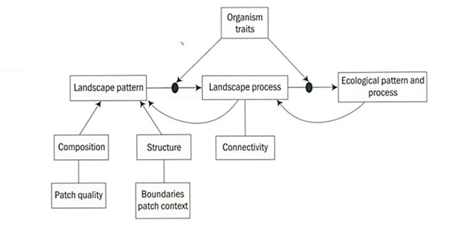 Figure 17.3. Conceptual Model of Landscape Pattern and Process
1.4. Modelling Catchment Hydrology
Investigation of hydrology of catchment involves an understanding of the individual hydrologic response units (H Us) through the interaction of land use (vegetation), soil, and climate in the determination of regional water balance (precipitation minus evapo¬transpiration) and resulting soil moisture, and partitioning of this balance between more rapid surface pathways for flow (run-off, subsurface pathways—through flow, groundwater recharge). In order to understand these response units, information about spatial distribution and topological network of connectivity of the hydrologic response units is required. The questions to be answered are as follows:
(i) Potential impacts of land cover and/or land-use change on water resources (the seasonal or long-term regime)
(ii) Impact of land-use change on soil and nutrient erosion, transport of point and non-point source contaminants, variations and change in aquatic or wetland environments, and associated biota (flora and fauna)
(iii) Impact on downstream, considering the lateral movement of surface and subsurface flows
Data required for catchment hydrologic modelling are as follows:
- The vegetation cover and land-use characteristics with spatial and temporal variation.
- Climatic characteristics (rainfall, temperature, humidity, and their variation with altitude) and spatial variations.
- Topological structure of their drainage network, which determines the lag time for arrival of rainfall to a point in the network, and the temporal concentration of the resulting stream flow hydrograph.
- Catchment's geomorphological and pedological characteristics and their spatial variation, which determine the potential for infiltration and local storage over run-off, and thus contribution to stream flow.
- Spatial distribution of inhabitants (population) in the catchment for assessing water demand. Location of population would determine the location of extractions and artificial storage of water from the channel network or from locally generated run-off and local groundwater sources. The location of population will determine the magnitude of local land-use change with corresponding impacts and the sources of point and non-point agricultural, industrial, and domestic pollution of the water sources.
1.5. Modelling Spatial Distribution of Selected Fauna Species: A Gis-Based Approach
Among the 25 global biodiversity hotspots, the Himalayan region and the Western—the two hotspots represented from India (Myers et al. 2000). The unique assemblages of flora and fauna in the Himalayan region make it one of the most important biodiversity hotspots. Seventy-five protected areas (PAs) encompassing 9.48 per cent of the region have been created to conserve this biodiversity and the fragile Himalayan landscape (Ruchi and Hussain 2003; World Conservation Monitoring Centre 1992.).
North-east India, the Western Ghats, and the north-western and eastern Himalayas are the regions of high endemism. Himalayan forests lie well north of the Tropic of Cancer. Some of them, at altitudes of 1,780-3,500 m are considered tropical forests since they occur within the climatic Tropics. The Himalayas have varied topography—a factor that influences and accommodates species diversity and endemism.
It is believed that forest cover in the Himalayas has dwindled from 340,000 sq. km, to 110,000 sq. km, with a mere 53,000 sq. km of primary forests. Despite this loss, the north-eastern region is home to some botanical rarities. One of these is the Sapria himalayana, a parasitic angiosperm that has been sighted only twice since 1836. This region is the meeting ground of the Indo-Malayan and Indo-Chinese bio-geographical realms, as well as the Himalayan and peninsular Indian elements, formed when the peninsular plate struck against the Asian landmass, after it broke off from Gondwana land. The numerous primitive angiosperm families found in this region include Magnoliaceae, Degeneriaceae, Himantandraceae, Eupomatiaceae, Winteraceae, Trochodendraceae, Tetracentraceae, and Lardizabaleaceae. The primitive genera are Almis, Aspidocarya, Belula, Decaisnea, Euptelea, Exbucklandia, Haematocarpus, Holboellia, Houttuynia, Magnolia, Mangelietia, Pycnarrhena, and Tetracentrol (Malhotra and Hajra 1977).
Despite being a biodiversity hotspot of the world with numerous endemic and endangered flora and fauna, the Indian Himalayan region is under threat from human-induced activities like hydropower projects, tourism, plantation crops, air pollution, etc. This has impacted on the landscape dynamics of the region, resulting in fragmented landscapes and forests.
Citation : T.V. Ramachandra, 2016, Ecological Modelling for Himalayas Guideline for BIO - GEO (Database Creation & Sustainable Watershed Development Planning in Himalayas) © Department of Science and Technology. Ministry of Science and Technology. Government of India, 2016 ISBN 978-81-7993-581-1