Summary: Ecological Carrying Capacity provides physical limits as the maximum rate of resource usage and discharge of waste that can be sustained for economic development in the region. This provides theoretical basis with practical relevance for the sustainable development of a region. Carrying capacity of a river basin refers to the maximum amount of water available naturally as stream flow, soil moisture etc., to meet ecological and social (domestic, irrigation and livestock) demands in a river basin. Monthly monitoring of hydrological parameters reveal that stream in the catchments with good forest (evergreen to semi-evergreen and moist deciduous forests) cover have reduced runoff as compared to catchments with poor forest covers. Runoff and thus erosion from plantation forests was higher from that of natural forests. Forested catchment have higher rates of infiltration as soil are more permeable due to enhanced microbial activities with  higher amounts of organic matter in the forest floor. Streams with good  native forest cover in the catchment showed good amount of dry season flow for all 12 months. While strems in the catchment dominated by agricultural and monoculture plantations (of Eucalyptus sp. and Acacia auriculiformis) are sesonal with water availability ranging between 4-6 months. This highlights the impacts of land use changes in tropical forests on dry season flows as the infiltration properties of the forest are critical on the available water partitioned between runoff and recharge (leading to increased dry season flows). This emphises the need for integrated watershed conservation approaches to ensure the sustained water yield in the streams. Assessment show that most Gram panchayats of Karwar and Bhatkal taluks, the Ghats of Supa, Ankola, Kumta, Honnawara, Siddapura, Sirsi and Yellapura have water for all 12 months (perennial). Gram panchayath in the coasts of Honnavara, Kumta and Ankola along with the Ghats of Siddapura, Sirsi, Yellapura and Supa towards the plains have water for 10 – 11 months, the plain regions of Haliyal and Mundgod taluks with part of Yellapura and Sirsi taluks show water availability for less than 9 months (intermittent and seasonal).

Quantification of silt yield highlights the linkage of silt yield with the land use in the respective sub-basin. Lower silt yield in sub-basins with good vegetation cover of thick forests, forest plantations, etc. The plains due to the higher lands under irrigation and are open lands, the silt yield is comparatively higher than that of other topographic regions. Strategies to regulate sand extraction are

Creation of No Development Zones (NDZ): Industries needs to be classified based on their type, and polices shall be amended upon which between 500 m to 10 km either sides of the river as listed in Table 4  and CRZ 1 (Coastal Regulation Zone 1).

Fixing of time for silt removal:  Removal of sand be permitted between 7 AM and 4 PM

Fixing of sand removal location and quantity: Based on category of river, sand removal shall be allowed only from the river bed, and no sand removal operation be allowed within 10 m of the river bank. No sand removal is allowed within 500 m from any bridge, irrigation project, pumping stations, retaining wall structures, religious places, etc.  Quantity of sand extracted at particular location shall not exceed the quantity of silt yield per annum.  Weighing bridges are to be fixed at identified locations to regulate the quantity of sand extracted during a year.

Fixing vehicle loading points:  Vehicles shall be parked at least 25 to 50 m away from the river banks, no vehicles shall be brought near the river bank. Erecting of pillars to demarcate vehicle restriction regions, beyond which vehicle should not be allowed

Restriction on mechanized removal: No pole scooping or any method shall be carried out in sand removal operation

Restriction or ban on sand removal: Sand shall not be removed from likely places where saline waters mixes with fresh water. Sand removal quantity per year based on scientific assessment and approval of on expert committee of district. Sustainable harvesting of sand considering the yield at point of extraction. Regions such as breeding habitat of fishes and other aquatic organisms, endemic species of riparian vegetation, and basins where ground water extraction is prevalent, are to be identified in the river basins for restricting sand mining. District collector may ban sand removal in any river or river stream during monsoons, based on the Expert Committee. Based on the acts, rules and orders made by the GOI/ state  the expert committee shall prepare river development plans for protection of river to keep up the biophysical environment along the river banks

Liability of District Collector: Fifty percent of the amount collected by the local authorities shall be contributed as river management fund and shall be maintained by the district collector.

No construction between 500 m to 1 km from flood plain: To protect life and property damages in cases of flash floods

Different stretch of rivers different regulations: Rivers are dynamic, they come across different geomorphic, climatic, sociopolitical settings. Due to this different stretches of rivers faces different issues. Rivers where rivers originate, they are at the highest purity level which needs to be maintained as it is the source contributor for the downstream.

Flood Plain protection: To protect against the damage that affects the floral and faunal diversity, intern maintaining the aesthetical and economic value of the river basins. No chemical based agriculture or fertilizers shall be used in the agricultural fields that affect the river channel polluting and affecting the ecosystem

 

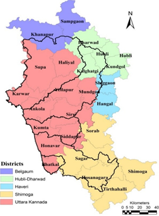
Keywords: Carrying capacity, river basin, silt yield

1.0 Introduction

Uttara Kannada is one of the ecologically sensitive districts of Karnataka State. It is one of the districts with the higher vegetation cover in India. Being situated on the Western Ghats, which is now considered one of the mega biodiversity regions of global importance has all the three major landscape system of the state namely; the coastal region on the west, the high hill mountain region of Sahyadri in the middle and a Deccan plateau margin in the eastern side. Due to factors like growing population and mega developmental projects, much of its natural landscape and the natural resource are under severe pressure in Uttara Kannada district. Deforestation, encroachment, submergence, forest fragmentation, river pollution and degradation and so many other impacts are already being witnessed. Keeping this fragile situation in mind, an integrated ecological carrying capacity study of the district was undertaken to provide the guidelines for the future conservation and sustainable development works.
Carrying capacity refers to the maximum number of activities (biological, developmental, agricultural, and industrial, population) that can be supported over a period of time in the habitat without damaging the existing quality of life, balance of resources, ecology and productivity of the ecosystem. Carrying Capacity provides physical limits as the maximum rate of resource usage and discharge of waste that can be sustained for economic development in the region. This provides theoretical basis with practical relevance for the sustainable development of a region. Carrying capacity of a river basin refers to the maximum amount of water available naturally as stream flow, soil moisture etc., to meet ecological and social (domestic, irrigation and livestock) demand in a river basin.

Carrying Capacity has been defined as the rate at which the resource can be consumed and discharged into the habitat without affecting the ecological integrity and biological productivity (MOEF, 2013, Subramanian 1998, Weizhuo Ji 2010, Jianhong Huang and Jing Cai 2011, Ying Li 2011, Ying Zhang et al 2009). The study of carrying capacity is carried out based on various aspects such as Population (Xilian Wang 2010, Subramanian 1998 ), Agriculture (Hegde 2012, Venkateswarlu and Prasad 2012, Masood Ali and Sanjeev Gupta 2012, Ghosh 2012), Industries (Subramanian 1998, Li Ming 2011), Livestock (Yu Long et al 2010, Gopal and Giridhari, 2000), Water and water bodies (Subramanian 1998, Li Ming 2011, Du Min et al 2011, Li-Hua Feng et al 2008, Connor et al 2001, Xie Fuju et al 2011), Forest, Soil (Xia and Shao 2008), Urban (Yuan Yan et al 2010, Peng Kang and Linyu Xu 2010), Mining (Xian Wei et al 2009), Marine (Hui Fu et al 2009), Ecotourism (Dan Luo and Nai'ang Wang 2010), Air (Goyal and Chalapati Rao 2011) etc.

Developing countries in the tropics are facing threats of rapid deforestation due to the unplanned developmental activities based on ad-hoc approaches and also due to lopsided policies that considers forest as national resource to be fully exploited. Anthropogenic activities coupled with skewed policies have resulted in the disappearance of pristine forests and wetlands in the form of logging, afforestation by plantation trees, dam constructions, and conversion of lands for other uses. This is evident from barren hilltops and increased spatial extent of barren or unproductive land. The structural changes in the ecosystem has affected the functional aspects namely hydrology, bio-geo chemical cycles and nutrient cycling. These are evident in many regions in the form of conversion of perennial streams to seasonal and disappearance of water bodies leading to a serious water crisis (Ramachandra et al., 2007; 2013a, b, c,d).. Thus, it is imperative to understand the causal factors responsible for changes in order to improve the hydrologic regime in a region. It has been observed that the hydrological variables are complexly related with the vegetation present in the catchment. The presence or absence of vegetation has a strong impact on the hydrological cycle. This requires understanding of hydrological components and its relation to the land use/land cover dynamics.  The reactions or the results are termed hydrological response and depends on the interplay between climatic, geological and land use variables (Ramachandra et al., 2007).

Burgeoning population with an enhanced demand of natural resources, there have been large scale over exploitation of natural resources such as water, forest, land etc. Changes in land cover leading to deforestation (Yong Lin and Xiaohua Wei 2008) and conversion to other land uses such as agriculture, horticulture, urban areas, etc., have affected the hydrological regime at regional scale (Ramachandra et al 2013d, Bonella et al 2010, Lin and Wei 2008). Large scale changes with increased open lands and agriculture land leads to higher water loss as runoff during the monsoon compared to forested landscape which has higher water holding capacity with sustained water supply during the post monsoon. The open lands and agriculture/horticulture fields, degraded forests lead to higher soil loss through erosion affecting the water holding capacity of the soils and crop productivity (Subramanian 1998). This necessitates an analysis and evolve apt management strategies to ensure sustenance of resources without losing its current potential. In any river basin, availability of water plays a prominent role in the productivity of forest and agriculture goods, while maintaining and restoring the ecological health in a basin (Faith Love et al 2006).  Thus for sustainable utilization of water in a region and to meet the demands of water optimally, it is necessary to assess the water resource carrying capacity (WRCC) considering the water availability and demand in a basin (Li Ming 2011, Du Min et al 2011, Faith Love et al 2006). WRCC is one of the key factors that define the limits up to which any developmental activities could take place without harming the regional or global ecology. The concept of ecological carrying capacity of a river basin integrates river basin management (Jing Li et al 2011) based on the basin structure and functional capabilities. The goal of the environmental water resource carrying capacity is to zone the river basins based on water quantity (flow) in the river basins that helps in the optimal management of water resources in the basin (Jing Li et al 2011, Das Gupta 2008) and identify the suitable developmental activities (Xu Ling 2011) based on the threshold in each zones. This also gives an opportunity to identify the basins/catchments that require an immediate attention of catchment restoration involving afforestation of location specific native species.

The flow in the river basin is quantified through discharge measurements in field associating with the volumetric analysis based on the hydro meteorological data using GIS and Remote Sensing (Chen and Zhao 2011). In any river, a minimum flow has to be maintained within a river, wetland, or coastal zone to maintain the functional abilities of ecosystems and the benefits they provide to people and the environment, these flows area referred to as ecological flows or environmental flow (Chen and Zhao 2011, Das Gupta 2008, Ramachandra et al., 2007; 2013). “Environmental flows” relate to protecting a range of environmental and community values including ecological systems, cultural and social values, recreational values and other amenity value; “Ecological flows” relate only to protecting specific ecological components , ecosystem health and/or functioning/processes (http://www.mfe.govt.nz). The process of ecological flow is being studied in many countries and also across countries such as China (Chen and Zhao 2011, Zhu and Yan 2011), India (Das Gupta 2008; Ramachandra et al., 2007; 2013d), Spain (Jorge Alcazar and Antoni Palau and Palau 2010), Tanzania (Japhet Kashaigili 2005), Korea (Woo 2010), Russia-China-Kazakhstan (Fucheng Yang et al 2012), South Africa (Hughes 2001), and many more. Analysis of environmental flow in streams and rivers are necessary to ensure that the need of humans and that of environment are met, based on which other potential users such as industries etc., can be accommodated to abstract water (Hughes 2001), in determining the health of river (Yang et al 2012), manage flow and protect the water bodies and river networks (Chen and Zhao 2011), maintain and enhance the ecological character and functions of floodplain, wetland and riverine ecosystems that may be subject to stress from drought, climate change or water resource development (ICUN 2011, Neil and Matthew 2012).

The study of ecological carrying capacity based on the ecological flow in each of the river basin of Uttara Kannada has been carried out by integration of the hydrological model with a water balance model and remote sensing data into a GIS (Neil and Matthew 2012, Mallikarjuna et al 2013, Ramachandra et al., 2007; 2013d). Remote sensing technique (Lillesand 2004, Sudhira et al 2004, Ramachandra et al 2012a, b, c) has advantages such as wider synoptic coverage of the earth surface with varied temporal, spatial and spectral resolutions. Classifications of these data through already proven classification algorithms (Ramachandra et al 2007; 2012a, b, Vinay et al 2012) provide land use information. Land use information derived from remote sensing is integrated through with the hydro-meteorological information to study the water balance in the respective basin. The hydro-meteorological studies and analysis has been carried out as per the standard protocol using the remote sensing data and other associated parameters such as rainfall, runoff, evaporation, transpiration, ground water monitoring and so on in determining famine, drought, cyclones, silt, flood monitoring etc. comparable to earlier work in Krishna basin (India-WRIS http://india-wris.nrsc.gov.in, Amoghavarsha et al 2012, Mallikarjuna et al 2013), Western Ghats (Ramachandra et al 2004, Ramachandra et al 2012a, Ramachandra et al 2013a, b, c, d, Reshma  et al 2012), Cauvery river basin (Vaithiyanathan et al 1992), etc. The hydrological parameters were transformed to spatial layers of the basin for assessing the carrying capacity in each sub-basin, based on the water budgeting (Peter 2002, Subramanya 2005, Raghunath 1985, Ramachandra et al., 2007).

The current study highlights the ecological carrying capacity of river basins of Uttara Kannada district of Karnataka. River basins were subdivided into sub- basins based on the tributaries. The sub basins were classified based on the flow in the  third order streams, and based on the supply of water as a function of rainfall and losses, demand based on the domestic water needs, crop water needs and  livestock water requirement. The water supply and water demand is used to identify the hydrological status of the river basins and flow assessment is carried out to identify the perennial and non-perennial streams in the river basin.   

2.0 Study Area
Uttara Kannada District located (at74005’13” - 75005’58” E and 13055’26” - 15031’23” N) towards the centre of the Western Ghats, along the coast of Karnataka has geographical area of about 10,280 sq.km (Figure 1). It is a region of gentle undulating hills, rising steeply from a narrow coastal strip bordering the Arabian Sea to a plateau at an altitude of 500 m with occasional hills rising above 600–860 m. It is surrounded by Belgaum District and State of Goa in the North, by Dharwar District in the East, Shimoga and Udupi Districts in the South. Arabian Sea forms the West border. The district capital is at Karwar. The district has 11 taluks covering three different zones i.e. coastal lands (Karwar, Ankola, Kumta, Honnavar and Bhatkal taluks), Sahyadrian interior (Supa, Yellapur, Sirsi and Siddapur taluks) and the eastern margin plains (Haliyal, Yellapur and Mundgod taluks). According to 2011 census the ppopulation of district is 14, 36, 847 and population density is 140 persons per sq. km. There has been 10.9 % increase in population density  from 118 (1991) to 132 (2011) persons per sq. km. 

There are five west flowing rivers namely Kali, Gangavali, Agnashini, Sharavathi and Venkatapura (Figure 1) and two east flowing rivers Dharma and Varada. These river basins extend from N 13043’4” to N 15033’38” Latitude and E 7504’54” to E 75019’52” Longitude, and are spread across neighboring districts such as Belgaum, Hubli, Dharwad, Haveri and Shimoga (Figure 2, Table 1). Ecological carrying capacity of major river basins have been done considering respective catchment (which extend beyond the political boundary of the district, listed in Table 1). The decadal population (aggregate of all river basins, beyond Uttara Kannada) has increased from 2071675 in 2001, to 2327710 in 2011 with a decadal increase of 12.4%. The population density has increased from 118 persons per square kilometer to 166 persons per square kilometer. At Basin level, population of Gangavali has the highest population, whereas Venkatapura highest population density with Kali being the lowest (Figure 3). These rivers give raise to magnificent waterfalls in the district. The Jog fall drops by 259 meters in Sharavathi, Lushington falls drops 116 meters in Aghanashini, Magod falls, where the Bedti river plunges 180 meters in two leaps, Shivganga falls, where the river Sonda (Bedthi) drops 74 meters, and Lalguli and Mailmane falls on the river Kali. Kali river origins in Joida taluk flows through Karwar taluk, Gangavali (Bedthi) origins in Dharwad District flows through Yellapur and Ankola taluks. Aghanashini river origins in Sirsi flows through Siddapur and Kumta taluks. Sharavati origins in Shimoga district, which forms the famous Jog Falls flows through Honnavar (Ramachandra et al., 2013c).
Figure 1: Study area – Major river basins in Uttara Kannada district, Karnataka State, India

 

Figure 2: Rivers with their catchment (and respective regional administrative boundaries)

Figure 3: Basin wise population

With tropical climate the region receives an average annual rainfall in the range of 700mm at the plains in the north east to more than 5500 mm at the Ghats; the coasts receive annual rainfall of 3000 to 4000 mm. The maximum amount of rainfall is received during the month of June, July, August and September due to the South west monsoon (Ramachandra et al., 2013c, District at a glance 2011 – 2012 of Various Districts, Reshma et al 2012). The year may broadly be classified into four seasons. The dry season is from January to February with clear and bright weather. It is followed by hot weather from March to May. During this season thunderstorms are common in the month of May. On an average, temperature in the region varies from 15.40C during January to about 35.620C in April.

Table 1: River basins with the spatial extent and respective administrative regions

3.0 Method
3.1 Land Use Land Cover Dynamics: Land use Land cover (LULC) dynamics is a major concern, as the abrupt changes has a negative impact on ecology, climate, hydrological regime, ecological flow, and also people’s livelihood in the region. LULC dynamics are specific to a region and vary from region to region. Land Cover refers to the observed physical cover on the earth’s surface. Land cover essentially distinguishes the region under vegetation with that of non-vegetation. Land use refers to use of the land surface through modifications by humans and natural phenomena. Land use can be classified into various classes such as water bodies, built up, forests, agriculture, open lands, sand, soil, etc. Land use modifications alter the structure of the landscape and hence the functional ability of the landscape. The modification includes conversion of forest lands, scrublands to agricultural fields, and cultivation lands to built-up, construction of storage structures for water bodies leading to submergence of land features that may vary from small scale to large scale.

Landscape is heterogeneous land area of interacting systems which forms an interconnected system called ecosystem (Forman and Gordron, 1986). The functional aspects (interaction of spatial elements, cycling of water and nutrients, bio-geo-chemical cycles) of an ecosystem depends on its structure (size, shape, and configuration) and constituent’s spatial patterns (linear, regular, aggregated). The status of a Land use land cover can be visualized using the LULC information. Land use land cover information of a region provides a base for accounting the natural resources availability and its utilization. The information pertaining to LULC provides a framework for decision making towards sustainable natural resources management sensors (Ramachandra et al 2013b, c).

Satellite remote sensing technology provide consistent measurements of landscape condition, allowing detection of both abrupt changes and slow trends over time for managing natural resources (Kennedy et al. 2009; Fraser et al., 2009). Remote Sensing (RS) data with Geographic Information System (GIS) and Global Positioning System (GPS) helps in effective measure of landscape dynamics in cost effective manner (Lillesand et al., 2004, Ramachandra et al., 2012, 2013b,c,d). Method involved in classification of a remotely sensed data is depicted in Figure 4.  

Data Acquisition involves collection of the remotely sensed satellite data, ancillary data include cadastral revenue maps (1:6000), the Survey of India (SOI) topographic maps (1:50000 and 1:250000 scales), vegetation map of South India developed by French Institute (1986) of scale 1:250000. Remote sensing data IRS P6 LISS IV and LISS III data with a spatial resolution of 5.8 m and 23.5 m respectively for the year 2010 were used for the analysis, along with the Cartosat DEM of 30 m spatial resolution. Topographic maps provided ground control points (GCP’s) to rectify remote sensing data and scanned paper maps. French institute maps were delineated to identify the forest cover and used to classify the RS data. Other ancillary data includes land cover maps, administration boundary data, transportation data (road network), etc. Pre-calibrated GPS (Global Positioning System - Garmin GPS units) were used for field data collection, which were used for RS data preprocessing, classification as well as for validation.

Pre-processing of data: The remote sensing data is checked for radiometric errors and geometric errors, the radiometric errors are rectified through radiometric correction, and the image is geometrically rectified by geo-referencing the image. Geo-registration of remote sensing data has been done using ground control points collected from the field using pre calibrated GPS  and also from known points (such as road intersections, etc.) collected from geo-referenced topographic maps published by the Survey of India. The geo-referenced image is cropped to the study area. Vector data of the district, taluk, river basins and village boundaries, drainage network, water bodies (lakes, ponds) were digitized from the Survey of India topographic maps, cadastral maps and digital elevation models. Population census and taluk wise village boundaries were collected from the Directorate of Census Operations (http://censuskarnataka.gov.in). 

Figure 4: Method of LULC analysis

Land use classification and accuracy assessment: This involved i) generation of False Colour Composite (FCC) of remote sensing data (bands – green, red and NIR). FCC helped in locating heterogeneous patches in the landscape ii) selection of training polygons covering 15% of the study area and uniformly distributed over the entire study area, iii) loading these training polygons co-ordinates into pre-calibrated GPS, vi) collection of the corresponding attribute data (land use types) for these polygons from the field, iv) Supplementing this information with Google Earth/Bhuvan. Land use classification was done using supervised pattern classifier - Gaussian maximum likelihood algorithm based on various classification decisions using probability and cost functions Land uses during the different period were computed using the temporal remote sensing data through open source GIS: GRASS- Geographic Resource Analysis Support System (http://ces.iisc.ernet.in/grass). The land use was classified into eleven groups such as Built up, Water, Agriculture, Open spaces, Moist Deciduous forest, Semi evergreen to evergreen forest, Scrub and Grass land, Acacia / Eucalyptus plantations, Teak / Bamboo plantations, Coconut/ Arecanut plantations and Dry Deciduous. 60% of the derived signatures (training polygons) were used for classification and the rest for validation. Statistical assessment of classifier performance based on the performance of spectral classification considering reference pixels is done which include computation of kappa (κ) statistics.

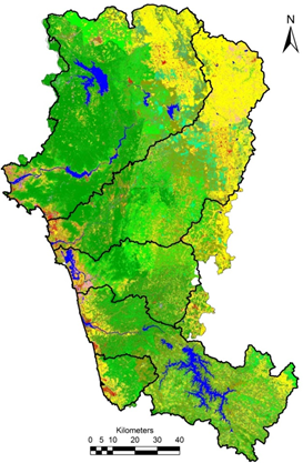
Figure 5: River basin wise Land use

Land uses in the respective river basins of Uttara Kannada district is given in Figure 5 and table 2. The urban landscape is about 1.9 % of the total area, and are prominent along the coast and plains, water bodies are about 3.1%, whereas the forest cover an area about 44.1 % with 28.6% of evergreen species and 15.5% of deciduous species. The overall classification accuracy was 91.51% with agreement (kappa) of 0.90.

 

Table 2: Land use categories with spatial extent

3.2 Quantification of Hydrological Regime: Sub-basin wise hydrological assessment for major rivers of Uttara Kannada has been done using land use information with meteorological and lithological parameters.  Figure 5 outlines the method adopted for assessing the hydrological parameters and water budgeting with ecological flows.

Water Balance: Sub-basin wise water balance (WB) is a function of water availability (WA) and water demand (WD) and is given by equation 1.
WB = f(WA,WD)         …..1
Where,  WB  =  Water balance, WA = Water available, WD = Water demand
The water availability in the sub basin depends on hydro-meteorological factors (Raghunath 2005) and demographics (land use, slope, soil…etc.) of the region, where as the water demand depends on the irrigation, domestic and livestock water requirements along with evapotranspiration. In any river basin if WA is less than WD, then this condition in the river basin during the month can be referred to as water deficit period.

Hydrological water balance (Peter 2002, Subramanya, 2005; Raghunath, 1985) equation is used to quantify the amount of water that goes through various phases of the Hydrological Cycle (Subramanya, 1994). The water balance equation is based on the law of conservation of matter (Raghunath, 1985) and is given by equation 2 (Subramanya, 2005; Raghunath, 1985).
Inflow = Outflow + ∆Storage.   ………2
Inflow into a river sub basin includes precipitation and groundwater discharge, whereas out flow from sub basin involves interception, surface runoff, pipe flow (lateral flow), transpiration, evaporation, groundwater recharge.

Figure 5: Method for hydrological assessment

Rainfall: Daily rainfall data of various rain gauge stations (point data) in and around the study area for the period 1901 to 2010 were considered to assess the trends of rainfall. The rainfall data used for the study were obtained from (a) Department of statistics, Government of Karnataka and (b) Indian metrological data (IMD), Government of India

Some rain gauge stations did not have complete rainfall records (rainfall details missing for few months). These missing data’s were evaluated through regression analysis and error data’s were revised with respect to neighboring rain gauge stations. This has been done as the analysis without considering the missing data gives erroneous results and also stations with missing rainfall cannot be included in the analysis. Rainfall trend analysis was done to understand the variability of rainfall at different locations in the study area.

Long term daily rainfall data were used to calculate the monthly and annual rainfall in each rain gauge station based on mean and standard deviation at selected rain gauge stations. The average monthly and annual rainfall data (point data) were used to derive spatial rainfall information for entire basin through interpolation (isohyets). The interpolated rainfall data was used to derive the gross yield (RG) in a respective basin (equation 3). Net yield (RN) was quantified as the difference between gross rainfall and interception (In), given in equation 4.

RG = AS * P          ……. 3
RN = RG – In       ………4

Where,  RG  =   Gross rainfall yield volume,   AS =   Area in Hectares, P  =  Precipitation in mm, RN =   Net rainfall yield volume and In  =   Interception volume
Rainy days and months per year was derived at each of the rain gauge stations considering two cases as:

• Case I : Rainfall more than 50 mm per month.
• Case II: Rainfall more than 100 mm per month.

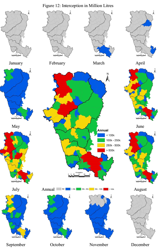
Interception: In any catchment, not all portions of rain reaches directly on to the ground as some portion of it is intercepted due to foliage, buildings and some is evaporated (returned back to the atmosphere without reaching the ground surface). This kind of water loss to atmosphere is referred as interception loss. Interception loss accounts to about 20% to 30% of the total seasonal precipitation. Table 3 gives the interception loss based on the vegetation in the Western Ghats.

*Source: Putty and Prasad, 2000
** Source: Modified evaporative fraction from Shuttleworth, 1993.

Interception is considered as a function of canopy storage capacity C and evaporative fraction (a) (Singh, 1992) as given by the equation 5. Interception based on vegetation types is listed in

I = C + α*P     …. 5

Table 4: Interception Equations for upstream River Basin

The rate of evaporation of intercepted water from a wet canopy commonly exceeds the potential evaporation for open water surfaces and depends on the locally available energy (Shuttleworth, 1993). The net amount of water, which the canopy can store, i.e. the interception storage capacity, depends partly on the nature of rainfall, in particular the intensity and duration of the rainstorm since up to 50% evaporation occurs during the storm itself. Intense, short-lived, convective storms, more common in tropical regions are associated with a lower fractional interception loss or evaporative fraction. Thus interception would be about 10-18 percent of precipitation (Lloyd et al., 1988; Shuttleworth, 1989) in forests with complete canopy cover. Storms associated with frontal rainfall, which may be less intense but lasts longer tend to give a higher fractional interception loss of say 20-30 percent of precipitation (Calder and Newson, 1979; Gash et al., 1980).     

The following assumptions have been made for interception loss under each vegetation type in the upstream of river basins. Major portion of the rainfall is received from the south west monsoon, which is of low intensity and longer duration. Thus, the evaporative fraction is considered similar to that of frontal precipitation.

Assumptions Vegetation type wise assumptions are:

Evergreen/semi-evergreen forests	Dominated by evergreen trees Leaves all year around- high storage capacity Thick and multi layered canopy- higher evaporative fraction
Moist deciduous forests	Dominated by deciduous trees Full leaves during monsoon season- maximum storage capacity Large leaves- higher evaporative fraction
Plantations	Dominated by monoculture trees Full leaves during monsoon season- maximum storage capacity Narrow and vertically aligned leaves- lower evaporative fraction
Agricultural crops	Young leaves (July-August)- lower storage capacity and evaporative fraction Mature leaves (September)- higher storage capacity and evaporative fraction
Grasslands and scrubs	Fully grown grass and scrubs-(June-September)- higher storage capacity and evaporative fraction Dry grass and scrubs (October)-lower storage capacity and evaporative fraction

 

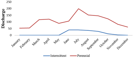
Runoff: Runoff is a process which involves draining off the precipitated water from a catchment into stream. Runoff represents the response of the catchment towards precipitation, climate and demographic characteristics. True runoff can be represented as the stream flow in natural conditions i.e., without any human intervention. Runoff can be characterized into two categories namely a) direct runoff or storm runoff and b) base flow.

Direct runoff is part of runoff that enters into the stream immediately after precipitation. During precipitation, portion of water gets percolated to the underlying strata (vadose and groundwater zones). Runoff in stream of a catchment dominated by vegetation begins on saturation of underlying strata of water. While, in open area or surface, without vegetation severe run off is observed, often as flash floods.

Base flow is the delayed water flow in the streams. This happens during post monsoon depending on the amount of water stored in the soil stratum (above the ground water table) and as ground water discharge (water stored in saturated / ground water zone). Plot of water discharge with time gives the hydrograph for a particular stream / river. Investigation of hydrographs enables one to classify the stream (Figure 6) as  (i) Perennial, (ii) Intermittent and (iii) Ephemeral

Figure 6: Stream classification depending on the duration of flow

The flow characteristic of the streams depends upon:

• Rainfall characteristics such as magnitude, intensity, distribution in time, space and variability.
• Catchment characteristics such as soil, vegetation, slope, geology, shape, drainage density
• Climatic factors such as temperature, humidity…etc.
• Infiltration depending on soil permeability.

Surface runoff has been determined by rational method, which assumes a suitable runoff coefficient to determine the catchment yield, which is given by equation 6:

Runoff = C * A * RN                         ………..6
RN       = RG – I     ………….. 4
Where
C   = Runoff coefficient, depends on the land use in the catchment (given in table 5)
A   = Area of catchment under different land use in square units
RN  = Net rainfall in mm
RG  = Gross rainfall in mm
I     = Interception in mm

Table 5: Land use and their surface runoff coefficients

Sub Surface Flow (Pipe flow): Pipe flow is considered to be the fraction of water that remains after infiltrated water satisfies the available water capacities under each soil. This corresponds to the amount of water stored in vadose zone (during precipitation). Pipe flow is estimated for all the basins as function of infiltration, ground water recharge and pipe flow coefficient as given in equation 7.

PF = (Inf – GWR) * KP                    ………7

Where              PF        = Pipe flow
Inf       = Infiltration volume
GWR   = Ground water recharge
KP        = Pipe flow coefficient (table 6)

Coefficients for pipe flow are determined from comparing the relief ratio of each sub basin. It has been observed that higher the relief ratio, lower the pipe flow coefficients and vice versa (Putty and Prasad, 2000). Table 6 lists coefficients considered based on relief ratio (Ramachandra et al., 2007). Observed pipe flows were related to the forest vegetation cover in the respective sub-basins: forests up to 50% of the area, pipe flow was observed to be 0.1 indicating higher water holding capacity in the region.

Infiltration: Infiltration is the process of water percolating the soil surface by action of gravity. Portion of the infiltered water is stored as soil moisture and in vadose zone and ground water zones. This water gets released to the respective streams during lean seasons (after monsoon season). As runoff recedes in the stream, water stored in vadose zones moves laterally, as stream flow. Then water stored in ground water zone would  be the water available in streams. Portion of water getting in streams, referred as base flow depends on the amount of water stored during monsoon. This depends upon the land use in the basin, precipitation rate, soil characteristics, slope, drainage density, etc. Infiltration is estimated as a difference between net rainfall yield (RN) to Runoff (equation 8)

Inf = RN – Runoff                 ….…8

Where,   Inf     = Infiltration Volume
RN     = Net Rainfall Yield (Volume)
Runoff         = Runoff Volume

Ground Water Recharge: Recharge is considered the fraction of infiltrated water that recharges the aquifer / ground water zone. After saturation of groundwater zone, water gets stored in vadose zone. Ground water recharge is given by equation 9 (Krishna Rao, 1970).

GWR = RC * (RN – C) * A   ……….9

Where 
GWR   = Ground water recharge
RC        = Ground water recharge coefficient, depending on the amount of annual rainfall, as given in table 7
RN        = Net Rainfall in mm
C         = Rainfall Coefficient,   A      = Area of the catchment

The recharge coefficient and the constant vary from location to location based on the annual rainfall.

Table 7: Ground water recharge coefficients

Groundwater Discharge: Groundwater discharge or base flow is estimated by multiplying the average specific yield of aquifer under each land use with the recharged water (equation 10). Specific yield represents the water yielded from water bearing material. In other words, it is the ratio of the volume of water that the material (after being saturated), will yield by gravity to its own volume. Base flow appears with the receding of pipe flow in a stream. Pipe flow and base flow sustains water flow in a river during the dry season.

Groundwater storage-discharge is considered to be linear (Maillet, 1905, Wittenburg and Sivapalan, 1999). The exponential function has been widely used to describe base flow recession, where Qt is discharge at time ‘t’ and Q0 is the initial discharge and a is a recession constant. The exponential function describes that the groundwater aquifer behaves like a single linear reservoir with storage linearly proportional to outflow i.e. 

                                                                S =a*Q          ……. 10      

    This equation represents a first order process or an exhaustion phenomenon expressed by
                                                                                                                    
                                                                Q(0)= Q0

The most widely used base flow recession equations,  given below (Barnes, 1939).     

                        Qt = Q0 *kt                     …… 11                       

                               
Where,             Q0- initial discharge
k – Base flow recession constant (0.85-0.99) (Subramanya, 2005).
t - Time
In absence of discharge data, volumes can be used. Replacing discharge with volume does not change its form and is less sensitive to errors (Singh, 1992). This is useful for partitioning surface and sub-surface flows (Shirmohammadi et al., 1984). Groundwater volume at any time‘t’ is determined by equation 12.

Vt = Vo * k t          ……..12      

                              
Assumptions

• The entire river basin is considered to be an unconfined aquifer
• Base flow recession constant is assumed to be 0.95

Based on the basin characteristics and rock type, ground water discharges for different basins were characterized as a function of ground water recharge and specific yield (equation 13).

GWD = GWR * YS                        ……. 13

Where,             GWD = Ground water discharge
GWR   = Ground water recharge
YS        = Specific yield, depending on rock type (table 8)

3.3 Supply: During monsoon and in the initial stages, water supply is a function of runoff in the respective stream in each sub-basin.  Water available as surface run off during monsoon, while the water stored in underlying strata (vadose and ground water zones) moves laterally to

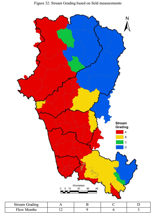
the stream during non-monsoon. Water recharge potential and discharge potential is a cumulative of monthly potentials during monsoon and is used during runoff deficits.

Stream Characterization: Stream discharge is the rate at which a volume of water passes through a cross section per unit of time. It is expressed in cubic meters per second (m3/s) or cumecs. The velocity - area method using current meter was used for estimating discharge. The cup type current meter was used in a section of a stream, in which water flows smoothly with velocity reasonably uniform in the cross section. A cross-section was chosen where the current was reasonably regular over the whole width. This measurement was done for three consecutive days every month for 36 months and 5 readings were taken at each point in order to take into account day-to-day fluctuations and seasonal variations. Table 9 lists stream wise flow and relative grading of streams (as A, B, C and D) depending on the availability of water in a stream.

Table 9: Stream flow data for major tributaries of streams

Stream	Location	Stream flow measurement (Discharge m3/sec)				Stream Grading*
		Oct.	Nov.	Dec.	Jan
Nandiholé	Northeast	01.23	03.68	0.09	0	D
Haridravathi	East	16.23	03.02	0.46	0	D
Mavinaholé	East	05.93	03.00	0.44	0	D
Sharavathi	Southeast	26.73	5.83	1.08	0.964	C
Hilkunji	Southeast	46.27	10.64	2.64	1.67	B
Nagodiholé	West	22.56	4.84	1.90	1.42	A
Hurliholé	West	06.30	1.37	0.78	0.661	A
Yenneholé	West	NM	13.40	1.81	1.68	A

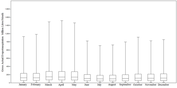
3.4 Water Demand: Water demand in each basin is calculated as the sum of Domestic demand, Livestock demand, Crop water requirement and Evapotranspiration for each month (Equation 14).
Water demand = Evapotranspiration  + Crop Water Requirement + Domestic water demand + Livestock water demand       …… 14

Evapotranspiration: Evapotranspiration is the total water lost from different land use due to evaporation from soil, water and transpiration by vegetation. Transpiration is the process by which water escapes to atmosphere as vapour from plants through leaves and other parts above ground. The water is taken from ground (soil) through the roots. On the other hand, evaporation continues throughout the day and night at different rates (Subramanya 2005, Birhanu et al 1995). The process of evaporation takes place on all land uses (other than vegetation). Some of the important factors that affect the rate of evapotranspiration are (Dunn and Mackay 1995, Raghunath 1985, Subramanya 2005) Atmospheric vapour pressure, precipitation, temperature, wind, light intensity, sunlight hours, humidity, plant characteristics (roots, steam and leave system, growth phase), soil moisture, etc.

If sufficient moisture is available to completely meet the needs of vegetation in the catchment, the resulting evapotranspiration is termed as potential evapotranspiration (PET), PET is also defined as the rate of evapotranspiration from an extensive surface of 8 to 15 cm tall, green grass cover of uniform height, actively growing, completely shading the ground and not short of water (Bapuji et al 2012). The real evapotranspiration occurring in specific situation is called as actual evapotranspiration (AET). These evapotranspiration rates from forests are more difficult to estimate than for other vegetation types. The difficulty in estimation arises because the turbulent diffusion in the atmosphere above the forests is much more efficient than for crops. For this reason, the rate of evaporation when the canopy is wet can be much greater than when it is dry. Thus, it becomes necessary to separate transpiration from evaporation of rainfall by forest canopy rather than considering the average effect of controlling processes within the canopy in terms of a single (effective) surface resistance (Shuttlewoth, 1993).

Potential evapotranspiration (PET) is determined using Hargreaves method (Hargreaves, 1972, Xu and Singh, 2004; Xu and Singh, 2005, Alexandris et al 2008) an empirical based radiation based equation (equation 15), which is shown to perform well in humid climates. PET is estimated as mm using the Hargreaves equation is given as

PET = 0.0023 * (RA/λ) *  *          …..15

Where              RA        = Extra-terrestrial radiation (MJ/m2/day)
Tmax   = Maximum temperature
Tmin    = Minimum temperature
λ          = latent heat of vapourisation of water (2.501 MJ/kg)

Actual evapotranspiration is estimated as a product of Potential evapotranspiration (PET) and Evapotranspiration coefficient (KC) as in equation 16. Evapotranspiration coefficient is a function of land use varies with respect to different land use (FAO, Marvin 2010, Stan et al 2001, Venkatesh et al 2011) and are listed in Table 10.

AET = PET * KC                  …….. 16

Table 10: Evapotranspiration coefficient

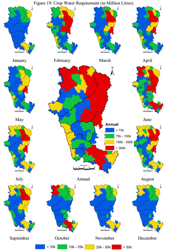
As the crop water requirement was estimated for different crops and different seasons based on land use, assumption is individual crop water requirement based on their different growth phases need different quantum of water for their development inclusive of evaporation.

Crop Water Requirement: The crop water requirement for each crop type based on their growth phases were used to determine the crop water requirement under each river sub basins. Crop water requirement is computed basin-wise as per equation 17.

Crop water Requirement (monthly) = Σ (Area under each crop * Crop water required for each crop) in a basin       …..17

Spatial extent of each crop (agriculture, horticulture) under irrigation for each sub basin was computed (as part of land use analysis) using remote sensing data. District at a glance 2011-2012 of all the covering districts was used to determine taluk-wise area under different types of crops. This information was used to estimate the area under each type in each sub basin.  Crop water requirement for individual crops based on their sowing period and growth phases were based on field estimates and literatures (http://nfsm.gov.in/ - National Food Security Mission,  http://krishisewa.com - Krishiseva Agriculture Information Hub, http://www.ikisan.com/ - IKisan Agriculture portal, http://www.iari.res.in  - Indian Agriculture Research Institute, http://eands.dacnet.nic.in - Directorate of Economics and Statistics http://www.bounteouskarnataka.com - Bounteous Karnataka, http://www.fao.org - FAO‎. The crop water requirement under each crops include water losses due to transpiration loses during their growth phase. Crop water requirement (kilo litres per hectare) under various crops based on their growth period are listed in Tables 11a and 11b respectively.

Table 11a: Cropping season and water requirement (cum per crop per ha)

Table 11b: Crop Water Requirement (cum per crop per ha)

Domestic water requirement: This is the water required for domestic purposes (cooking, bathing, etc.) in the river basin. Domestic water requirement is calculated as product of water required per person per day and population in the basin. Population for the year 2013 was computed using the growth rate based on the population of 1991, 2001 and 2011 for each village. Aggregation of villages, provided the population for the respective sub basin.

Pn = Pn-1 * (1 + n*r)      …….18

Where
Pn = Estimated population for the current year
Pn-1 = Earlier population (Census)
n = number of decades
r = population growth rate
Domestic water requirement is computed for each basin considering the population and per capita daily water requirement and number of days in  a month (equation 19).

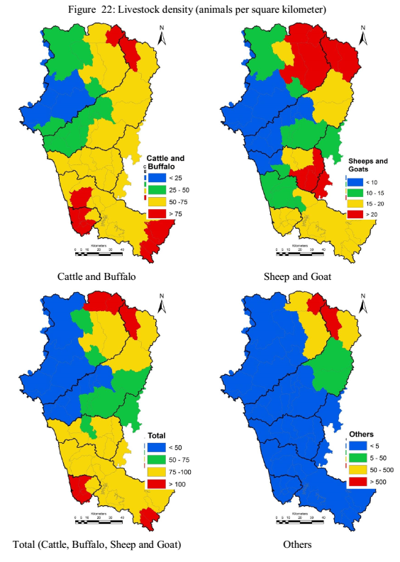
Domestic Water Required = Population * per capitaDaily Water Requirement * Number of day in a month ……. 19

The domestic water requirement in India varies from season to season and also from urban to rural areas (India Water Portal, http://www.indiawaterportal.org, National Institute of Hydrology, http://www.nih.ernet.in). On an average Daily water requirement during various seasons are; Summer 150lpcd, Monsoon 120 lpcd, Winter 135 lpcd.

Livestock water requirement: Livestock water demand is estimated as the product of livestock population and monthly water requirements under each category of livestock (equation 20). Taluk wise livestock population was acquired from the publication - District at a glance 2011-2012.

Livestock Water Required = Livestock Population * Daily Water Requirement * Number of day in a month             ………20

Daily water requirement varies depending on the season and animal type (table 12).

Table 12: Livestock water requirement

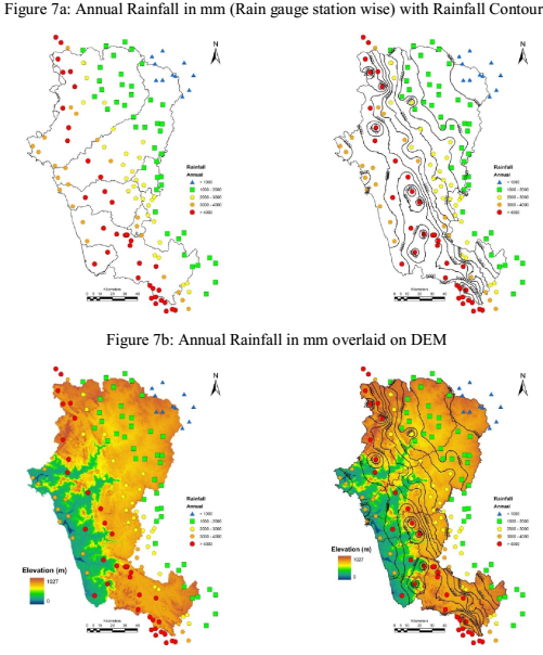
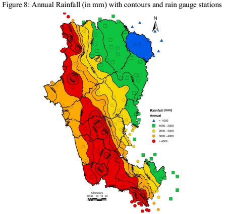
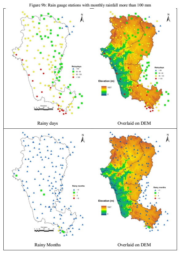
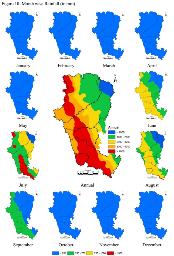
The livestock water requirement for the above animals were derived through telephonic interviews with the locals and experts apart from published literatures (http://www2.ca.uky.edu/ - University of Kentucky, http://www.nature.com - Nature, , North http://www.ncsu.edu - California State University.

3.5 Water balance: Depending on the supply and demand of water, hydrological status of a sub-basin is computed. Hydrologic status is the ratio of  water supply to  water demand. If the is less than 1, the basin is said to be  water deficit, otherwise surplus. If the ratio falls below 0.3 then there is very low flow or no flow in stream. Flow in stream is categorized as perennial (A – type, all 12 months water) or seasonal  (B – water for 9 months, C: 6 months water flow and D – 4 months or only during monsoon).

4.0 Results and Discussions:
4.1: Water availability / supply

Rainfall: Rainfall analysis was carried out using daily rainfall data  for the period 1901 and 2010 of 144 Rain gauge stations in and around the study area (covering all sub basins of major rivers in Uttara Kannada). Mean annual rainfall ranges from 550 mm (in the plains towards Hubli-Dharwad District) to over 6500 mm (in the Ghats of Sagara and Hosanagara taluks of Shimoga district). Within the region, rainfall varies between 750 mm to over 5500 mm. Figure 7a indicates the annual rainfall distribution across the region.  Ghats section with thick forest cover receives annual rainfall of over 4000 mm, whereas the coast receives annual rainfall between 3000mm to 4000 mm and the plains with moderate forests receive annual rainfall between 1000 to 3000 mm (Figure 7b). Plains with no/very little forest cover or scrubs receive very low annual rainfall of less than 1000 mm. Figure 8 shows annual rainfall received in the whole catchment by interpolating the rainfall (rain gauge station) and isohyets.

Forest vegetation depend on the quantity of rainfall and number of rainy days/wet days. Number of rainy days computed, rain gauge station wise considering rainfall (i) more than 50 mm/month and (ii) more than 100 mm/month. Figure 9a and figure 9b shows the spatial distribution of rainy days and rainy months on an average in a year for both cases. For both the cases coasts and the Ghats receive rainfall for over 90 days in a year, indicating higher annual rainfall, good vegetation (forest) cover and high variations in terrain at these rain gauge stations, rainy months at these rain gauge stations are over 6 months in both cases, and extend over 8 months when rainfall is over 50 mm per month. With terrain getting flatter and less undulating towards the plains, the rainfall intensity decreases with less dense or degraded vegetation (forest) cover, the number of rainy days dropdown to less than 90, and 6 or less rainy months in an year in both cases, and drops to 2 months in case of rainfall less than 100 mm/month in parts of Hubli and Dharwad. The plains in the north east receives rainfall in 2 rainy seasons, one during the south west monsoon, the other during north east which results in higher rainy months/days. Sub basins surrounding the dam sites and large lakes receive local rains during summer, observed near Linganamakki reservoir of the sharavathi river basin, at Supa, Bommanhalli, Tattihalla, Kadra, Kaneri and Kodsalli dam sites of Kali basin, and Gangavali basin respectively.  Monthly rainfall given in figure 10 shows higher rainfall during monsoon months between June and September, with maximum rainfall during July.

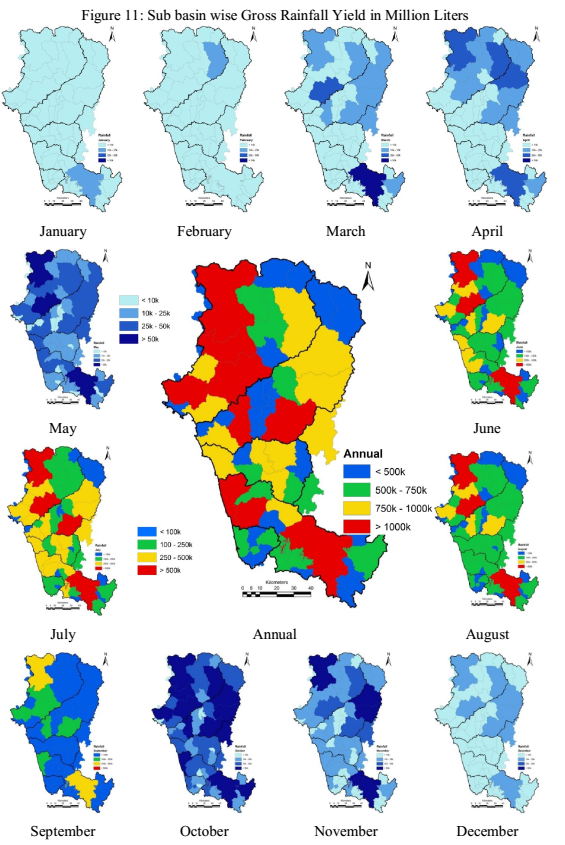
Sub basin wise distribution of gross rainfall is given in figure 11. Gross rainfall is the product of precipitation and area under each sub basin, and the rainfall yield depends on the spatial extent of sub-basin. Some sub-basin shows higher values even in cases when the rainfall is low due to the large spatial extent of the respective basin. Interception in figure 12 for each basins is based on the regional land use and precipitation. The region with denser canopy cover has higher interception losses; the intercepted water contributes to evaporation during monsoon. Net rainfall is depicted in figure 13, is the difference between the gross rainfall and interception.

 

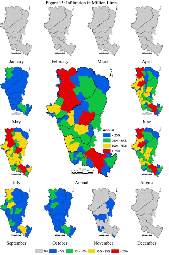
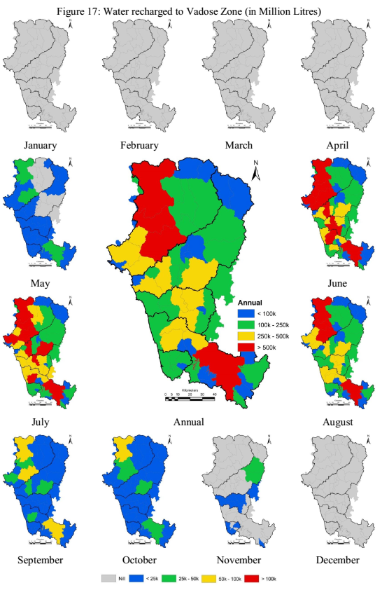
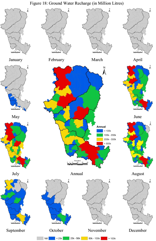
Runoff: Runoff assessment was carried out using the empirical equation as a function of land use, precipitation (more than 50 mm/month) and area of sub basin. Monthly runoff is given in figure 14. Runoff in the basins begins in May (at coast of Uttara Kannada and Ghats of Shimoga) and continues till October. Runoff is high in the streams towards the plains (in the north east) due to no/low vegetation cover. Basins with thick vegetation have less runoff coefficients and higher water holding capabilities (as in Ghats). Despite high rainfall, runoff is moderate due to thick vegetation cover. Dam sites also indicate higher runoff during monsoon (annual). Runoff is one of the major causes for flow in streams during monsoon and along the downstream during post monsoon when stored in reservoirs.

Infiltration: Infiltration in each of the river sub-basins were assessed as function of net rainfall and runoff and is depicted in figure 15. Basins with higher vegetation cover show higher infiltration capacity compared to open areas and buildups. Higher infiltration / percolation is due to soil being porous due to organic matter and associated microbial action. Also, catchment with good vegetation cover have higher stream density compared to catchment with open area (sparse stream density).

Base flow: Base flow in each basin indicated is as indicated in figure 16, is assessed as function of infiltration. Base flow is very high in basins with reservoirs, as the ground water table is high and soil layers are over saturated, allowing larger amount of water to drain through the soil stratum into the streams.

Sub-surface flow: Sub-surface flow happens when adequate water is stored in vadose zone during rainfall. Figure 17 shows the water recharge capacity into the vadose zone. Apart from the basins with major reservoir’s, the Ghats have higher water holding capacity of soils since they receive higher amount of rainfall, as these regions also have higher vegetation covered with diverse endemic and non-endemic floral species.

Ground Water Recharge: Ground water recharge potential for different river sub basins, month wise is given in figure 18, based on soil and lithology with rainfall of over 100 mm per month. The Ghats receive highest rainfall resulting higher ground water recharge potential, followed by coasts.

4.2 Water Demand
Crop water requirement: Sub-basin wise irrigation crop water requirement is computed and presented in figure 19. Sub-basins in Ghats indicate lesser irrigation and horticulture water requirement. Rain fed paddy is grown in this region. Sub basins with two season rice crops indicate higher water requirement. In sub basin toward Hubli-Dharwad district, cash crops are grown indicating higher water requirement. The crop water requirement is high in the north and north east in the plains, followed by coast, followed by the Ghats.
Domestic water requirement: the water requirement is function of population, and water requirement per person in the particular season. Population in the basin for the year 2013 was estimated using the earlier census for each river sub basin. Figure 20 indicates the population density (persons per square kilometer).  Table 12 indicate the increase in population density since 1991.
Table 12: Population density variation in each sub basins

Of the five river basins, Venkatapura basin has the highest population density of about 309.84 persons per square kilometer followed by  Gangavali (198.77), Kali (155.91), Aghanashini (146.10) and Sharavathi (108.92) basins.  Domestic water requirement of each sub basin is given in figure 21.  Coast and the plains show higher domestic water requirement due to higher population, whereas the Ghats indicate low domestic water requirement due to lower population.
Livestock Water Requirement: Livestock population density for each of the basins and for different livestock categories as shown in figure 22. The plains in the north east have higher sheep and goat population density as these basins have longer dry months with less rainfall. Whereas the coasts (Bhatkal taluk) of venkatapura river basin have higher cattle and buffalo density. Similar to domestic water requirement, livestock water requirement is computed and given in figure 22. Due to higher animal population, larger livestock water is required in the plains along the north east, east, followed by the coast in the west and Ghats in the north of the study area.

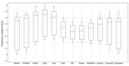
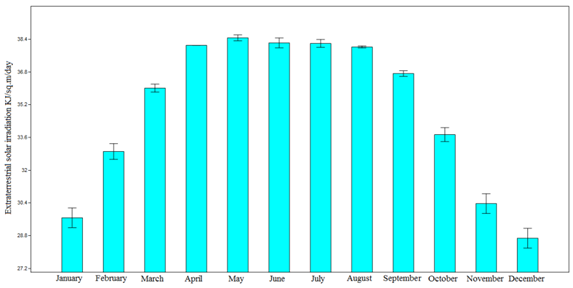
Potential Evapotranspiration: Potential evapotranspiration was estimated using Hargreaves method. Figure 24 depicts month-wise PET variations, which ranges from 5.6 mm/day (May) to 2.8 mm/day (July). Supplementary data to estimate PET are temperature (figure 25) (www.worldclim.org) and extraterrestrial solar radiation data (figure 26). Temperature in the basin on an average varies from as low as 15.4 °C (January) to 35.62 °C (April). Extraterrestrial solar irradiation depends upon the locations (latitude and longitude), and its position above or below the equator. It varies from 28.12 KJ/m2/day (December) to about 38.63 KJ/m2/day (May).

Figure 24: Month-wise Potential Evapotranspiration (mm/day)

Figure 25:  Month-wise Temperature (°C)

Figure 26: Extraterrestrial solar radiation (KJ/m2/day)

Figure 27: Gross AET Million Litres

Gross Actual evapotranspiration is derived as product of evapotranspiration coefficient and PET, is depicted in figure 27, indicating higher values during April, and lower values during July.  Net Evapotranspiration is derived as difference between gross actual evapotranspiration and interception, as interception losses account to evapotranspiration and is as shown in figure 28. The evapotranspiration losses during monsoon is due to the process of interception of water. Higher forest cover in the Ghats contribute more to evapotranspiration loss. Sub basins with large water bodies contribute to a higher evapotranspiration followed by basins covered with dense forests.

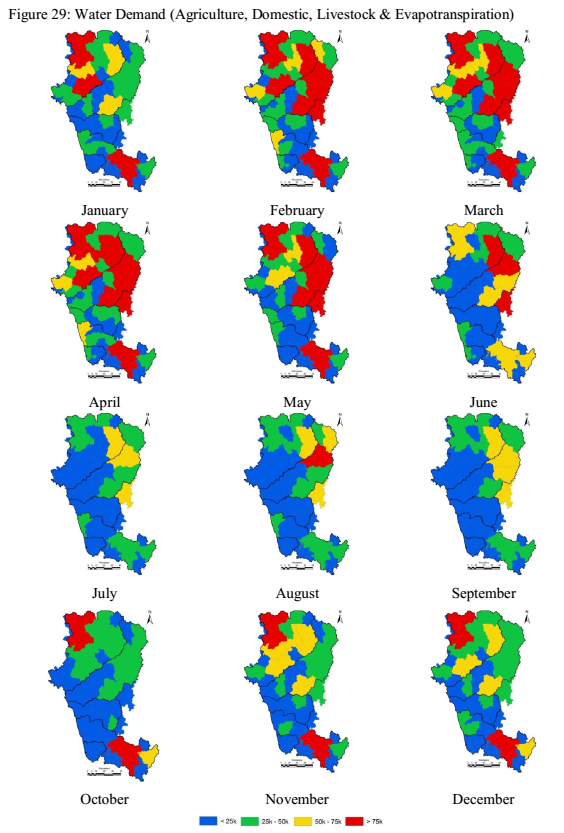
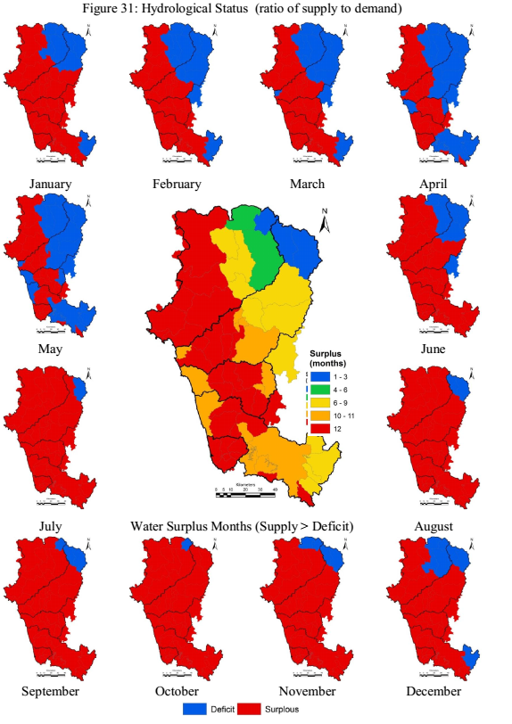
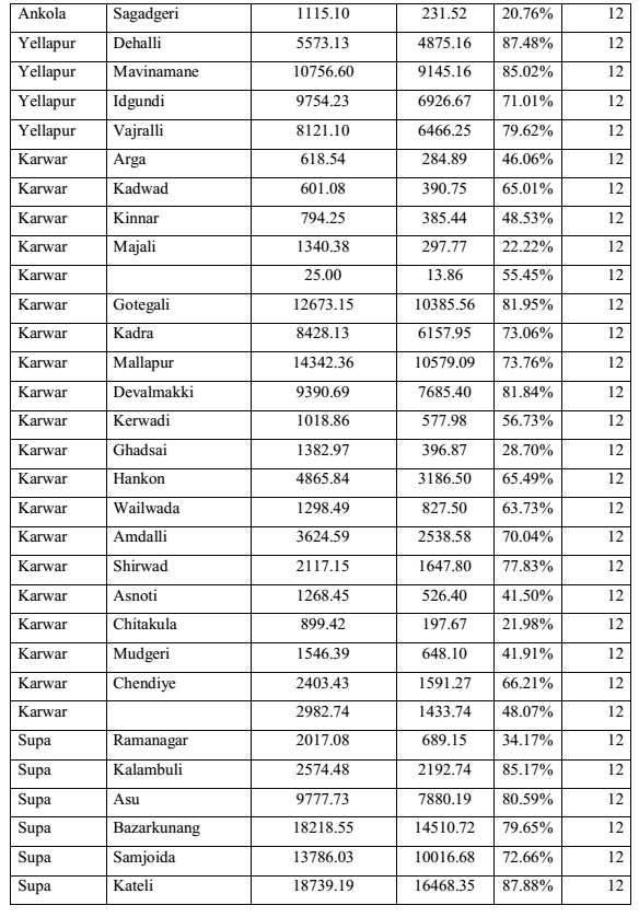
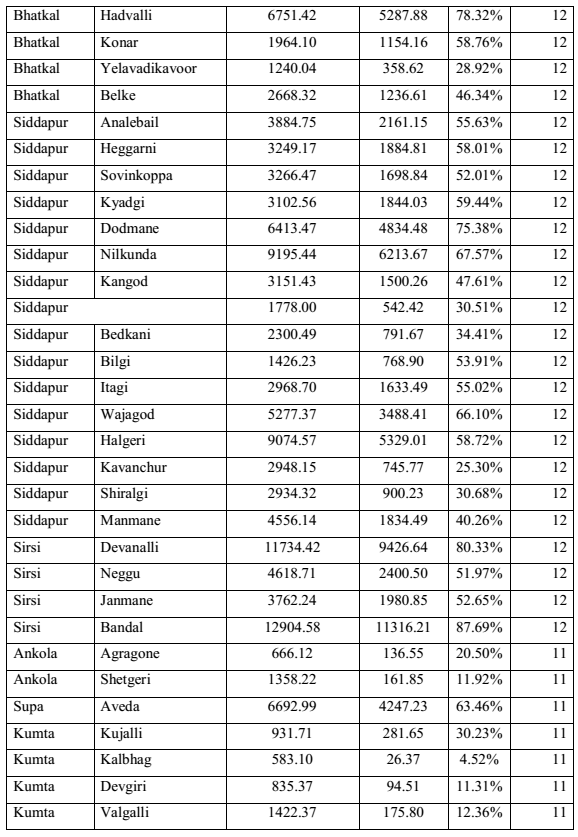
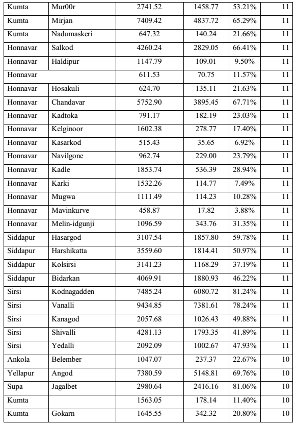
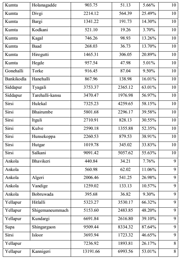
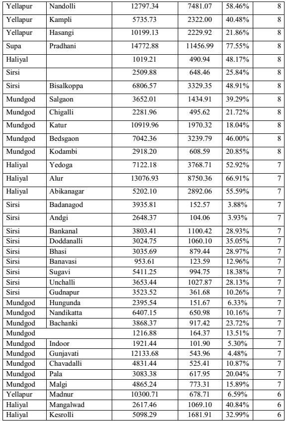
Total Water Demand: Total water demand is the combination of crop water requirement, domestic and livestock water demand, and evapotranspiration. The total water demand given in figure 29, indicates of higher demand during dry seasons. The Northeastern part of the study area in the basins of Kali and Gangavali has a higher water demand, whereas the demand is comparatively less in Ghats, and regions dominant with natural vegetation cover. 

Water Availability: Water supplied to cater the demand varies with the water available as runoff, vadose water and ground water discharge. Figure 30 shows the season wise water availability. During, December to May in some of the river sub basins of Kali, Gangavali and Sharavathi, water availability falls to zero indicating non-availability of naturally available water sources in the sub basin.

5.0 Water Budget and Stream flow assessment:  Figure 31 indicates the hydrological status highlighting the basins with the water availability as either surplus or deficit (scarce). If the ratio of availability to demand falls below 1, sub-basin indicates the scarcity of water. Figure 31 also highlight the water availability as number of months in a year. The Ghats and some part of coast (with good forest cover) show water availability during all 12 months, whereas some sub-basins towards the plains and the rest of the coast the surplus is available between 6 to 11 months and the plains has the water available for less than 6 months

Streams were graded as A, B, C and D depending on the perennial, intermittent or seasonal water availability (which are comparable to field measurements, table 9). Figure 32 highlights the hydrological status of all rivers in Uttara Kannada district.

Figure 33 shows the Gram panchayat wise hydrological status. Most Gram panchayats of Karwar and Bhatkal taluks, the Ghats of Supa, Ankola, Kumta, Honnawara, Siddapura, Sirsi and Yellapura have water for all 12 months (perennial). Gram panchayath in the coasts of Honnavara, Kumta and Ankola along with the Ghats of Siddapura, Sirsi, Yellapura and Supa towards the plains have water for 10 – 11 months, the plain regions of Haliyal and Mundgod taluks with part of Yellapura and Sirsi taluks show water availability for less than 9 months (intermittent and seasonal). Table 13 below shows the forest cover in each of the Gram panchyayat’s along with the water availability as surplus in months.

4.5: Relationship between flow regime and the parameters affecting the flow
Step wise multiple regression analysis was carried out to find the probable relationship between various parameters that would contribute to the flow of water in the rivers (Table 14).
Flow regime Fl = f(Rainfall, Runoff, Slope, land use, base flow, pipe flow, etc) … 21
The flow regime is a physical phenomenon that is dependent upon basic aspects such as the slope, land use, drainage density, and rainfall; and derived aspects such as runoff, pipe flow, Pipe Flow, forest cover and type of forest such as interior forests, perforated forests, patch forests, edge forests, and transitional forests
Table 14: Probable relationship between flow regime and environmental variables

Fl: Flow regime in months;  Pnet: Net Rainfall in mm; R : Runoff in mm; V : Vadose in mm; Pf: Pipe flow in mm; Gwd: Ground water discharge in mm; S: Slope as percentage; E: Elevation in meters; Dd: Drainage density as per meter; AH: Combined Agriculture and Horticulture as percentage; FP: Forest plantation as percentage; AP: Agriculture plantation as percentage; F: Total forest as percentage; If: Interior forest as percentage; Pef: Perforated forest as percentage; Paf: Patch forest as percentage; Ef: Edge forest as percentage; Tf: Transition forest as percentage;
The significance value for all the above relationships were less than 0.05, indicating good confidence level of 95 % of the relationships. The relation between runoff, ground water discharge, interior forest and perforated forest provides significant results with coefficient of determination as 0.802. i.e.,
Fl = 0.0034 * R + 0.0086 * Gwd + 7.571 * If + 20.092 *Pef + 1.740  …..42
The equation indicates that the presence of interior forest has higher importance over the flow regime, as forests hold higher water in vadose and ground water zones and releases water during lean season to streams as pipe flow or base flow.

References

1. Subramanya K, 2005, Engineering Hydrology, Tata McGraw-Hill publishing company limited New Delhi, Second Edition. ISBN: 0-07-462449-8
2. Raghunath H M, 1985, Hydrology, Wiley Eastern Limited, ISBN: 0-85226-746-0
3. Raghunath H M, 2005, Ground water, New age international publishers, Second Edition ISBN: 0-85226-298-1
4. Peter S Eagleton, 2002, Ecohydrology – Darwin in expression of vegetation form nad function, Cambridge university press, ISBN: 0-521-77245-1
5. National Institute of Hydrology, http://www.nih.ernet.in
6. Hydraulic Design Manual, http://onlinemanuals.txdot.gov/txdotmanuals/hyd/rational_method.htm
7. Ananth kumar, 2012, Integrated basin management studies in Sitanadi basin, Western Ghats region, Karnataka, India Water Week 2012 – Water, Energy and Food Security: Call for Solutions, 10-14 April 2012, New Delhi.
8. Rainfall-Runoff modeling of Western Ghats region of Karnataka, National institute of hydrology, CS(AR)-31/98-99
9. http://www.waterboards.ca.gov/water_issues/programs/swamp/docs/cwt/guidance/513.pdf
10. http://www.fao.org
11. http://ces.iisc.ernet.in/energy/water/proceed/section7/paper5/section7paper5.htm
12. http://www.slideshare.net/cpkumar/estimation-of-groundwater-potential-2490240
13. Xu C Y and Singh V P, 2000, Evaluation and generalization of radiation-based methods for calculating evaporation, Hydrological processes, Vol.14, pp 339-349
14. Xu C Y and Singh V P, 2001, Evaluation and generalization of temperature-based methods for calculating evaporation, Hydrological processes, Vol.15, pp 305-319
15. Birhanu Zemadim , Felix Mtalo, Simon Mkhandi, Raj Kachroo and Matthew McCartney, 2011, Evaporation Modelling in Data Scarce Tropical Region of the Eastern Arc Mountain Catchments of Tanzania, Nile Basin Water Science & Engineering Journal, Vol.4(1), pp 1 - 13
16. Dunn S M and Mackay R , 1995, Spatial  variation  in  evapotranspiration  and  the  influence  of land  use  on  catchment  hydrology, Journal  of  Hydrology,  Vol.171, pp 49-73
17. Bapuji Rao B, Sandeep V M, Rao V U M and Venkateswarlu B, 2012, Potential Evapotranspiration estimation for Indian conditions: Improving accuracy through calibration coefficients, National Initiative on Climate Resilient Agricultre, Tech. Bull. No. 1/2012.
18. Alexandris S, Stricevic R and Petkovic S, 2008, Comparitive analysis of reference evapotranspiration from the surface of rainfed grass in central Serbia, calculated by six empherical methods against the Penman- Monteith formula,European Water21/22, pp 17-28
19. Marvin Jensen E, 2010, Estimating evaporation from water surfaces, CSU/ARS Evapotranspiration Workshop, Fort Collins, CO, 15-Mar-2010
20. Stan Wullschleger D, Hanson P J and Todd D E, 2001, Transpiration from a multi-species deciduous forest as estimated by xylem sap flow techniques, Forest Ecology and Management,Vol.143, pp 205-213
21. Venkatesh B,   Lakshman Nandagiri,   Purandara B K and  Reddy V B, 2011, Modeling Soil Moisture under different land covers in a sub-humid environment of Western Ghats, India, Journal of Earth System Science , Vol.120 (3), pp 387-398
22. National Food Security Mission , http://nfsm.gov.in/nfsmmis/RPT/CalenderReport.aspx
23. Krishiseva Agriculture Information Hub, http://krishisewa.com/cms/crops-calendar.html
24. IKisan Agriculture portal, http://www.ikisan.com/
25. Indian Agriculture Research Institute, www.iari.res.in
26. Directorate of Economics and Statistics, Department of Agriculture and Cooperation, Ministry of Agriculture, Government of India, eands.dacnet.nic.in/At_A_Glance-2011/Appendix-IV.xls
27. Bounteous Karnataka, Government of Karnataka, www.bounteouskarnataka.com/DP-PDF/DistrictProfile-UttaraKannada.pdf. ‎
28. http://censusindia.gov.in/
29. Uttaara Kannada District at a glance, 2011-2012
30. www.worldclim.org
31. Ministry of Environment and forest, http://envfor.nic.in/
32. Subramanian D K, 1998, A framework for conducting carrying capacity studies for Dakshina kannada district, IISc Archive
33. Ying Zhang, Taihai Xu, Zhao Jiang, Xinran Peng, Lin Zhang and Shuang Kang, 2009, Quantitative Calculation Models and the Application of Ecological Carrying Capacity, IEEE Xplore, pp 1-3
34. Xilian Wang, 2010, Research Review of the Ecological Carrying Capacity, Journal of Sustainable Development, Vol. 3(3), pp 263 – 265.
35. Hegde D M, 2012, Carrying capacity of Indian agriculture: oilseeds, Current Science, Vol. 102(6), pp 867-873.
36. Venkateswarlu B and Prasad J V N S, 2012, Carrying capacity of Indian agriculture: issues related to rainfed agriculture, Current Science, Vol.102(6), pp 882 – 888
37. Masood Ali and Sanjeev Gupta, 2012, Carrying capacity of Indian agriculture: pulse crops, Current Science, Vol.102(6), pp 874 – 881
38. Ghosh S P, 2012, Carrying capacity of Indian horticulture, Current Science, Vol.102(6), pp 889 – 893
39. Li Ming, 2011, The Prediction and Analysis of Water Resource Carrying Capacity in Chongqing Metropolitan, China, Procedia Environmental Sciences, Vol.10, pp 2233 – 2239
40. Yuan Yan, Li  Li and Li Yankui, 2010, An  Analysis  of  Environment  and  Resources Carrying  Capacity  for  Guiding  Urban  Planning: A Case  Study  of  Hezhou,  China, 2nd  Conference on  Environmental  Science  and  Information  Application Technology-2010, IEEE, pp 235 – 238
41. Xian Wei, Zhou Wancun and Shao Huaiyong, 2009, Study on the Ecological Carrying Capacity in Mining Areas: A case Study in Panxi Mining Concentrated Area, The 1st International Conference on Information Science and Engineering (ICISE2009), IEEE Computer Society, pp 2193 – 2197.
42. Hui Fu, Yijie Liu and Yinglan Sun, 2009, A Study on the Marine Ecological Carrying Capacity in Qingdao Based on Principle Component Analysis and Entropy, IEEE Xplore, pp 1-4
43. Dan Luo and Nai'ang Wang, 2010, Assessment of environmental carrying capacity of ecotourism for Maqu, 201O International Conference on Computer Application and System Modeling (ICCASM 2010), IEEE, Vol.15, pp 518 – 520.
44. Weizhuo Ji, 2010, Dynamic Analysis of Ecological Footprint and Ecological Carrying Capacity, 2010 Sixth International Conference on Natural Computation (ICNC 2010), IEEE, pp 3033 – 3036
45. Jianhong Huang and Jing Cai, 2011, Analysis of Environmental Carrying Capacity of Hainan against the Background of Island Economy, IEEE, pp 8054 – 8057.
46. Yizhong Zhu and Shilu Yan, 2011, Estimate of Eco-environment Carrying Capacity of Guangzhou, IEEE Xplore, pp 1 – 4
47. Du Min, Xu Zhenghe, Peng Limin, Zhu Yunhai and Xu Xiufeng, 2011, Comprehensive Evaluation of Water Resources Carrying Capacity of Jining City, Energy Procedia, Vol.5 ,pp 1654–1659
48. Goyal S K and Chalapati Rao C V, 2007, Air assimilative capacity-based environment friendly siting of new industries—A case study of Kochi region, India, Journal of Environmental Management, Vol. 84, pp 473–483
49. Li-Hua Feng, Xing-Cai Zhang and Gao-Yuan Luo, 2008, Application of system dynamics in analyzing the carrying capacity of water resources in Yiwu City, China, Mathematics and Computers in Simulation, Vol. 79, pp 269–278
50. Ying Li, Tingting Guo, and Jing Zhou, 2011, Research of Ecological Carrying Capacity -Comprehensive Evaluation Model, Procedia Environmental Sciences, Vol. 11, pp 864 – 868
51. Peng Kang and Linyu Xu, 2010, The urban ecological regulation based on ecological carrying capacity, Procedia Environmental Sciences, Vol. 2, pp 1692–1700
52. Xia Y Q and Shao M A, 2008, Soil water carrying capacity for vegetation: A hydrologic and biogeochemical process model solution, Ecological modeling, Vol. 214, pp 112–124
53. Yu Long, Zhou Li, ,Liu Wei and Zhou Hua Kun, 2010, Using Remote Sensing and GIS Technologies to Estimate Grass Yield and Livestock Carrying Capacity of Alpine Grasslands in Golog Prefecture, China, Pedosphere Vol. 20(3), pp 342–351
54. Gopal Thapa B and Giridhari Sharma Paudel, 2000, Evaluation of the livestock carrying capacity of land resources in the Hills of Nepal based on total digestive nutrient analysis, Agriculture, Ecosystems & Environment, Vol. 78(3), pp 223–235
55. Connor W P, Garcia A P, Connor A H, Garton E O, Groves P A and Chandler J A, 2001, Estimating the Carrying Capacity of the Snake River for Fall Chinook Salmon Redds, Northwest Science, Vol. 75(1), pp 363-371
56. Xie Fuju, Zjeng Mingx and  Zhang Hong, 2011, Research on Ecological Environmental Carrying Capacity in Yellow River Delta, Energy Procedia, Vol. 5, pp 1784–1790
57. Jing Li, Xiaode Zhou and Wen Chen, 2011, Study on Prince Edward River Basin’s Water Ecological Carrying Capacity based on Water Ecological District, IEEE Xplore, pp 1244-1249
58. Xu Ling, Liu Zhihong and Du Jing, 2011, Study on Evaluation of Water Ecological Carrying Capacity, 2010 International Conference on Biology, Environment and Chemistry, IPCBEE , Vol. 1, pp 458 – 462
59. Ramachnadra T V, Bharath H A and Vinay S, 2013, Land use Land Cover Dynamics in a rapidly urbanizing Landscape, SCIT journal (in press)
60. Faith Love, Elisha Madamombe, Brian Marshall and Evans Kaseke, 2006, Preliminary estimate of environmental flow requirements of the Rusape River, Zimbabwe, Physics and Chemistry of the Earth, Vol. 31, pp 864–869
61. Bonella M, Purandara B K, Venkatesh B, Jagdish Krishnaswamy, Acharya H A K, Singh U V, Jayakumar R and  Chappell N, 2010, The impact of forest use and reforestation on soil hydraulic conductivity in the Western Ghats of India: Implications for surface and sub-surface hydrology, Journal of Hydrology, Vol. 391, pp 47–62
62. Yong Lin and Xiaohua Wei, 2008, The impact of large-scale forest harvesting on hydrology in the Willow watershed of Central British Columbia, Journal of Hydrology, Vol. 359, pp 141–149
63. Chen H and Zhao Y W, 2011, Evaluating the environmental flows of China’s Wolonghu wetland and land use changes using a hydrological model, a water balance model, and remote sensing, Ecological Modelling, Vol. 222, pp 53–260.
64. Das Gupta A, 2008, Implication of environmental flows in river basin management, Physics and Chemistry of the Earth, Vol. 33, pp 298–303
65. Jorge Alcázar and Antoni Palau, 2010, Establishing environmental flow regimes in a Mediterranean watershed based on a regional classification , Journal of Hydrology, Vol. 388, pp 41–51
66. Japhet Kashaigili J, Reuben Kadigi M J, Bruce Lankford A, Henry Mahoo F and Damus Mashauri A, 2005, Environmental flows allocation in river basins: Exploring allocation challenges and options in the Great Ruaha River catchment in Tanzania, Physics and Chemistry of the Earth, Vol. 30, pp 689–697
67. Hyoseop Woo, 2010, Trends in ecological river engineering in Korea, Journal of Hydro-environment Research, Vol. 4, pp 269-278
68. Fucheng YANG, Ziqiang XIA, Lanlan YU and Lidan GUO, 2012, Calculation and Analysis of the Instream Ecological Flow for the Irtysh River, Procedia Engineering Vol. 28, pp 438 – 441
69. Hughes H A, 2001, Providing hydrological information and data analysis tools for the determination of ecological instream flow requirements for South African rivers, Journal of Hydrology, 241, 140–151
70. Lillesand M T, Kiefer W R, and Chipman W J, “Remote Sensing and Image Interpretation”, 5th ed. John Wiley and Sons. 2004
71. Sudhira H S, Ramachandra T V and Jagadish K S, 2004, Urban sprawl: metrics, dynamics and modelling using GIS. International Journal of Applied Earth Observation and Geoinformation, Vol. 5, pp 29-30.
72. Ramachandra T V, Bharath H A and Durgappa D S, 2012, Insights to urban dynamics through landscape spatial pattern analysis, International Journal of Applied Earth Observation and Geoinformation, Vol. 18, pp 329-343.
73. Ramachandra T V, and Bharath H A, 2012a, Spatio-Temporal Pattern of Landscape Dynamics in Shimoga, Tier II City, Karnataka State, India, International Journal of Emerging Technology and Advanced Engineering, Vol. 2(9) , pp 563-576.
74. Ramachandra T V, Bharath H A and Sreekantha S, 2012b, Spatial Metrics based Landscape Structure and Dynamics Assessment for an emerging Indian Megalopolis, International Journal of Advanced Research in Artificial Intelligence, Vol. 1(1), pp 48 – 57.
75. Indian Meteorological Department, http://www.imd.gov.in/
76. Vinay S, Bharath H A and Ramachandra T V, 2012, Spatio-temporal dynamics of Raichur City, LAKE 2012: National Conference on Conservation and Management of Wetland Ecosystems 06th – 09th November 2012
77. Neil Sims C and Matthew Colloff J, 2012, Remote sensing of vegetation responses to flooding of a semi-arid floodplain: Implications for monitoring ecological effects of environmental flows, Ecological Indicators, 18, 387–391.
78. India WRIS, http://india-wris.nrsc.gov.in/wrpinfo/index.php?title=Krishna
79. Amoghavarsha Murthy, Gouda K C, Reshma Bhat, Prabhuraj D K, and Lakshmikantha B P, 2012, Monitoring of 2009 Krishna River Flood using Remote Sensing and GIS, Proceedings of AGU Fall Meeting 2012, San Francisco, December 3rd - 7th  2012
80. Ramachandra T V, Subhash Chandran M D, Sreekantha, Diwakar Mesta, Rao G R and Sameer Ali , 2004, Cumulative impact assessment in sharavathi river basin, Internationan Journal of Environmental and Development, Vol. 1(1), pp 113 - 135
81. Ramachandra. T V, Subash Chandran M D, Joshi N V, Sreekantha, Raushan Kumar, Rajinikanth R, Desai S R and Subhash Babu, 2012c. Ecological Profile of Sharavathi River Basin., Sahyadri Conservation Series 22, ENVIS Technical Report : 52, November 2012, Energy & Wetlands Research Group, Centre for Ecological Sciences, Indian Institute of Science, Bangalore 560 012
82. Ramachandra T V, Subash Chandran M D, Surya Prakash Shenoy H, Rao G R, Vinay S, Vishnu Mukri and Sreekanth Naik, 2013a. Kumaradhara River Basin, Karnataka Western Ghats: Need for Conservation and Sustainable Use., Sahyadri Conservation Series 24, ENVIS Technical Report : 54, April 2013, Energy & Wetlands Research Group, Centre for Ecological Sciences, Indian Institute of Science, Bangalore 560 012.
83. India Water Portal, http://www.indiawaterportal.org/.
84. Reshma Bhat, Gouda K C, Amoghavarsha M, Lakshmikantha B P, Prabhuraj D K, 2012, Decadal Variation In The Rainfall Characteristics over River Basins across the Western Ghats of India, Proceedings of AGU Fall Meeting 2012, San Francisco, December 3rd - 7th  2012.
85. IUCN, 2011. eFlowNet Summary 2010. International Union for Conservation of Nature, http://cmsdata.iucn.org/downloads/newsletter_print.pdf
86. Vaithiyanathan P, Ramanathan A and Subramanian V, 1992, Sediment transport in the Cauvery River basin: sediment characteristics and controlling factors, Journal of Hydrology, Vol. 139(1–4), pp 197–210
87. Mallikarjuna V, Prasad K R K, Udaya Bhaskar P and Sai Lakshmi M, 2013, Water Balance Study of Krishna Delta, Andhra Pradesh, using GIS & RS Techniques, International Journal of Emerging Technology and Advanced Engineering, Vol. 3(6), pp 59 – 64
88. University of Kentucky, College of Agriculture Food and Environment, Lexington, http://www2.ca.uky.edu/poultryprofitability/Production_manual/Chapter12_Water_quality/Chapter12_introduction.html, table 12.1
89. Water Requirement of rabbits and Guinea Pigs, Nature, August 1943, V 152, pp-157 http://www.nature.com/nature/journal/v152/n3849/abs/152157b0.html
90. My Cocker Spaniel, http://mycockerspaniel.com/h2o.htm
91. North California State University, http://www.ncsu.edu/project/swine_extension/healthyhogs/book1995/almond.htm, table 1
92. http://www.mfe.govt.nz/laws/standards/ecological-flows-water-levels/workshops-ecological-flows-water-levels-faqs.html
93. Ramachandra T V, Subash Chandran M D,  Joshi N V and Bharath Setturu, 2013b, Land use changes with the implementation of developmental projects in Uttara Kannada district, Sahyadri Conservation Series 31, ENVIS Technical Report : 61, August 2013, Energy & Wetlands Research Group, Centre for Ecological Sciences, Indian Institute of Science, Bangalore 560 012.
94. Shimoga District at a Glance 2011 – 2012
95. Haveri District at a Glance 2011 – 2012
96. Belgaum District at a Glance 2011 – 2012
97. Dharwad District at a Glance 2011 – 2012
98. Ramachandra T V, Subash Chandran M D,  Joshi N V and Bharath Setturu, 2013c, Land use land cover (lulc) dynamics in Uttara Kannada district, central Western Ghats , Sahyadri Conservation Series 28, ENVIS Technical Report : 56, August 2013, Energy & Wetlands Research Group, Centre for Ecological Sciences, Indian Institute of Science, Bangalore 560 012.
99. Forman R T T and Gordron M., 1986. Landscape Ecology. John Wiley & Sons, New York, ISBN 0-471-87037-4.
100. Kennedy R E, Townsend P A, Gross J E, Cohen W B, Bolstad P, Wang Y Q and Adams P, 2009. Remote sensing change detection tools for natural resource managers: understanding concepts and tradeoffs in the design of landscape monitoring projects. Remote Sensing of Environment, Vol. 113, pp. 1382–1396.
101. Fraser R H, Olthof I, and Pouliot D, 2009. Monitoring land cover change and ecological integrity in Canada’s national parks, Remote Sensing of Environment, Vol. 113, pp. 1397–1409
102. Directorate of Census operations, Karnataka, http://censuskarnataka.gov.in
103. Ramachandra T.V., Subash Chandran M D., Gururaja K V and Sreekantha, 2007. Cumulative Environmental Impact Assessment, Nova Science Publishers, New York

1. [Author]

 

 

 

 

 

 

E-mail     |     Sahyadri     |     ENVIS     |     GRASS     |     Energy     |     CES     |     CST     |     CiSTUP     |     IISc     |     E-mail