SECTION 4 : ENVIRONMENT MONITORING IN THE NEIGHBOURHOOD
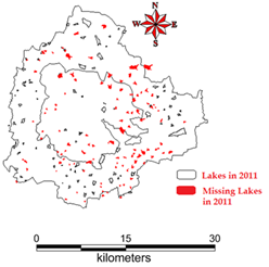
Environment monitoring is essential for evaluating environmental planning and policy. Long term monitoring helps in evaluating the success of policy as well as helps in identifying areas for improvement. Environmental monitoring provides a vital scientific insights of long-term trends apart from new knowledge and understanding. For Example, monitoring of Bangalore wetlands during the last two decades, provided evidence of poor environmental status of wetlands in Bangalore affecting the land and groundwater sources in the vicinity. Due to its distinctive contributions to science and practice, monitoring is an integral aspect of ecological research, management, and policy.
Environment monitoring in the neighbourhood would help in the preservation of natural resources (lakes, parks, street trees). During 2011-12, we attempted the deployment of student community from high schools and colleges to document biodiversity under the banner ‘My Village Biodiversity’ in the Uttara Kannada district of Karnataka State. This helped in the compilation of biodiversity information of 300 villages within a year. Competitions were conducted for students and nominal rewards announced for the best reports and good presentations. No financing of the educational institutions has been done to carry out this model of work. The objectives of environment monitoring is to generate “Environment Sensitive Citizens” required for the sustainable management of natural resources. This approach includes:
- Sensitisation of students: Pre testeddata formats is aimed at sensitizing students to environment, biodiversity and ecology related issues.
- Recording observations: Study and understand data formats necessary in the contemporary contexts of conservation and sustainable use. Regular monitoring would help in updating the environment information.
- Vital information on goods and service: documentation of goods and services and their significance in meeting the people’s livelihood.
- Low cost methods: long term monitoring would provide information and technique would be cost effective
- Creating ambassadors of goodwill: Students, with their unbiased minds were expected to merit greater acceptability in the neighbourhood, as the local people otherwise tend to be more reserved with outside agencies like NGOs engaged in such work.
- Expertise in communication:Students were expected to gain good communication skills.
- Capacity building: Students and teachers will have an opportunity to interact with the researchers from Indian Institute of Science, apart from taking active part in LAKE 2014 at Parisara Sabhangan, Sirsi, Uttara Kannada, Central Western Ghats during 13-15 November 2014 (details at the end of this report).
1.0 MAPPING AND MONITORING WATER BODIES
|
|
Bangalore city |
Greater Bangalore |
1973 |
58 |
207 |
2010 |
10 |
93 |
Objective: Mapping water bodies (Spatial extent and location)
Knowledge required: We need to know (i) Map (ii) Mapping tools (iii)Details about a Map
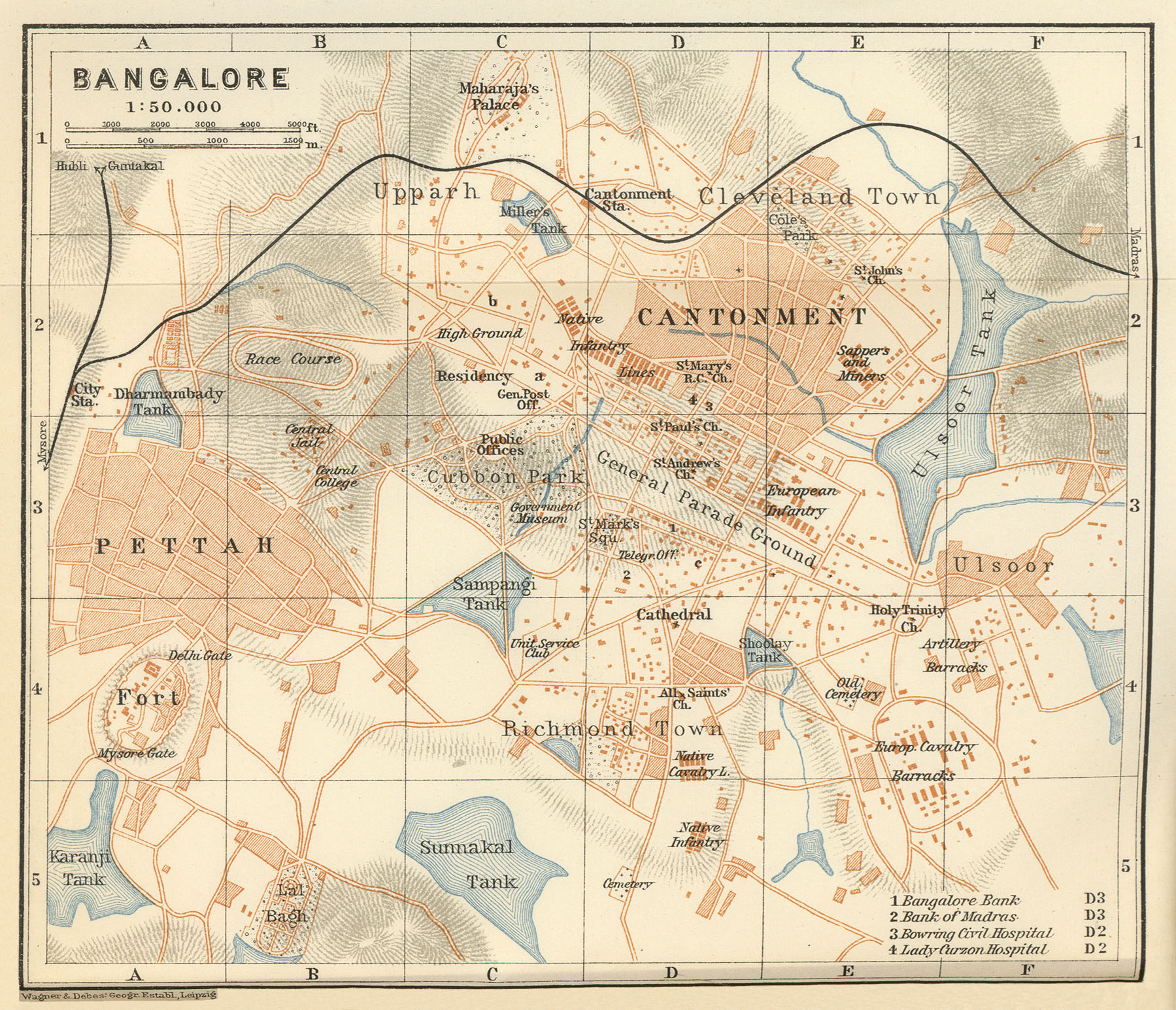
MAP: Is a diagrammatic representation usually on a flat surface of the whole or a part of the Earth surface showing various features like road, water bodies etc.
Types of Maps: Maps are classified based on (a) scale- On the basis of scale (ex. Cadastral Maps or Revenue Maps, Topographical Maps, Geographical Maps, Atlas Maps etc.,) (b) Contents and purpose (ex: Road map, Railway map, cultural map)
Cadastral Map
These maps are drawn on large scale ex: administration and collection of revenue
|
 Topographical Maps Topographical Maps
These maps show natural as well as man-made features of an area. |
 Geographical maps Geographical maps
They are on small scales in which strict representation of the individual features. |
How to read a MAP?
- North arrow represents North direction
- Scale is the ratio between distances on a map and the corresponding distances on the earth’s surface.
- Legend provides details of the content of the map.
Scale represents map unit on the ground. For example, scale of 1:250,000 means that 1 unit on the map corresponds to 250,000 units on ground.
Large scale means maps shows a larger details smaller area coverage (1:10,000). Gives details of each parcels of land |
Small scale maps means maps shows lesser details but large area covered |
Examples of Scales: 57/H/9/NE – 1:25000 map of North east area of Bangalore, 57/H/9 – 1:50000 Map of Bangalore,
Map: 57 indicate 1:1 million, 57/H -1:250,000 shows the district, 57– 1:100000 covers Indian subcontinent.
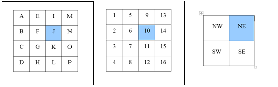
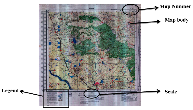
Map Numbering
57 - 40 x 40 on 1:1M scale Shaded cell shows 57 J of scale 1: 250000 |
57 - 10 x 10 on 1: 250000 scale Shaded cell shows 57 J/12 of scale 1:50000 scale |
57 - 15' x 15' on 1: 50000 scale Shaded cell shows 57 J/12/NE of scale 1:25000 scale |
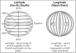
MAP Coordinate system: A coordinate system is a standardized method for assigning codes to locations so that locations can be found easily. Good example is Latitude (LAT) Longitude (long) system.
- Latitude: specifies the north-south position of a point on surface of Earth. Latitude is an angle which ranges from 0° at the Equator to 90° (North or South) at the poles. Reference being equator.
- Longitude: specifies the east-west position of a point on surface of Earth, measured as the angle east or west from the Greenwich Prime Meridian, ranging from 0° at the Prime Meridian to +180° eastward and −180° westward.
- Datum: A datum is a set of reference points on the earth's surface against which position measurements are made and an associated model of the shape of the earth to define a geographic coordinate system.
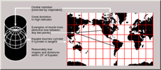
- Projection: A transformation of the spherical or ellipsoidal earth onto a flat map is called a map projection.ex: Projection: Cylindrical UTM projection as shown below, Datum:WGS84
Source: WIKI
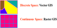
Spatial data: Data that represents the space is referred as spatial data. Two kinds of spatial data are (i) raster and (ii) vector. Both these are used in GIS (Geographic Information System) to store and retrieve geographical data.
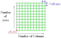
- Raster data: is a collection of cells which have a single value and are organized in arrays in number of rows and columns. Ex: Your own photograph is a raster data, when zoomed you can see pixels
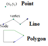
- Vector data: are associated with points, lines, or polygons, Points are located by coordinates, Lines are described by a series of connecting line segments and polygons are described by a series of vectors enclosing the area.
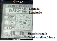
Global Positioning System (GPS): GPS help in locating the co-ordnates of a location, which helps in the navigation. This works on the constellation of 24 communication satellites. Minimum of three satellite signals are necessary for correct measurements.
- Switch on the GPS (Soft switch normally at top or front)
- Navigate to the page showing lat-long and satellite signal strength
- Stand in the location to be marked and press mark
- Note the waypoint number and lat-long and proceed
- GPS can also be connected to pc using USB and software
Conversion from Degree Decimals to Degree, Minutes, Seconds
Consider the example 96.31°, the whole units of degrees will remain the same (i.e. in 96.31°, longitude, start with 96°).
Multiply the decimal by 60 (i.e. .31 * 60 = 18.6).
The whole number becomes the minutes (18').
Take the remaining decimal and multiply by 60. (i.e. .6 * 60 = 36).
The resulting number becomes the seconds (36"). Seconds can remain as a decimal.
GPS NAME: ………………… Area surveyed…………………..
Date: …………………, Time: ………….., Name: ……………..
Location (inlet of lake, near place etc.) |
Waypoint number |
Latitude |
Longitude |
|
|
|
|
|
|
|
|
|
|
|
|
|
|
|
|
|
|
|
|
|
|
|
|
|
|
|
|
|
|
|
|
|
|
|
|
|
|
|
|
|
|
|
|
|
|
|
|
|
|
|
|
|
|
|
|
|
|
|
|
|
|
|
|
|
|
|
|
|
|
|
|
|
|
|
|
|
|
|
|
|
|
|
|
|
|
|
|
|
|
|
|
|
|
|
|
|
|
|
|
|
|
|
|
|
|
|
|
|
|
|
|
|
|
|
|
|
|
|
|
|
|
|
|
|
|
|
|
|
|
|
|

2.0 DIGITSING MAP FROM ONLINE DIGITAL DATABASE
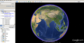
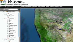
Google earth (http://earth.google.com) /Bhuvan (http://bhuvan.nrsc.gov.in)
Downloading Google earth
1. Go to http://www.google.com/earth/
2. Installing google earth : Click on downloaded googleearthupdatesetup.exe file to install, you will be greeted with below message
3. Creating a vector Layer (Polygon, Point, Line)
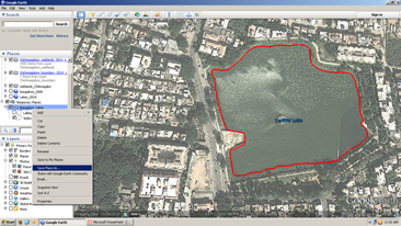
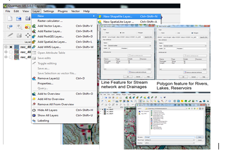
a. Adding a polygon – describes a area (ex boundary of a lake)

Use left mouse button to place points on boundary as shown below
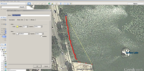
Once completed the entire waterbody click ok (example shown below)
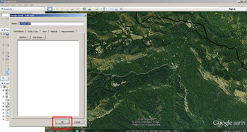
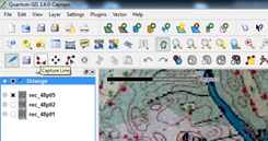
b. Creating a line feature to digitize a stream
Digitise river using mouse by left clicking at each point
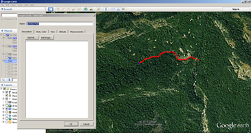
After entire stream is delineated click on ok
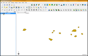
Example of first order streams and catchment delineated from Google earth
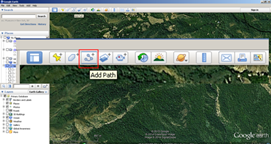
c. Creating a point feature to show a place of interest (Point may represent your school location)
Click on placemark as shown below

Click on ok, once you could locate your school
d. Save digitized KML layers : Right mouse click on the layer to be saved and select save place as
e. Select type as kml and press on button save as shown below
3.0 QUANTUM GIS (QGIS) – SPATIAL MAPPING TOOL
QGIS is a Free and Open Source GIS for manipulating geographical data (vector, raster), statistical analysis.
INSTALLATION:

- Click on download now you will find the list of versions available.
- Download the latest stable version.
- Installation of Software: Double click on QGIS-OSGeo4W-1.6.0-3-Setup-x86_32.exe. After the installation click on QGIS icon on the desktop.
Use of QGIS:
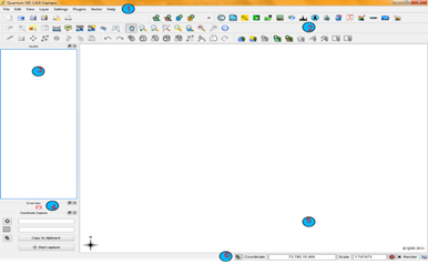
- QGIS main window will be opened and looks as shown
- The menu bar provides access to numerous QGIS features.
- The toolbars offers additional tools for interacting with the map. Hold the mouse over the particular icon, a short description of the tool’s purpose will be displayed.
- The map legend area sets the visibility
- QGIS - maps are displayed in map canvas area
- The map overview panel provides a full extent view of layers added
- The status bar shows the current position in map coordinates
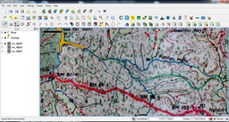
Geo referencing:
- Geo-referencing is the process of assigning real earth coordinates to the digitised maps, so it can be viewed, queried, and analysed with other geographic data.
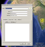
- To start geo referencing an unreferenced raster, we must load it by clicking Plugins menu option in the menu bar and click on Georeferencer plugin. The Georeferencer window will be opened click on File menu and click Add raster layer. The raster will show up in the main working area of the dialog. Once the raster layer is loaded, we can start to enter reference points.
- Using the Add Point button (Edità Add points), you can add points to the main working area and enter their coordinates. Click on a point in the raster image which you want to assign co-ordinates and enter the X and Y coordinates manually. With the move button option you can move the GCPs (Ground control points) on map, if they are at the wrong place.
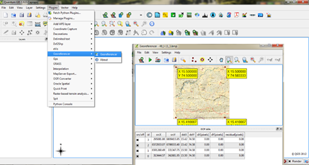
- Continue entering points. You should have at least 4 points and the more coordinates you can provide, the better the result will be. There are additional tools on the plugin dialog to zoom and pan the working area in order to locate a relevant set of GCP points.
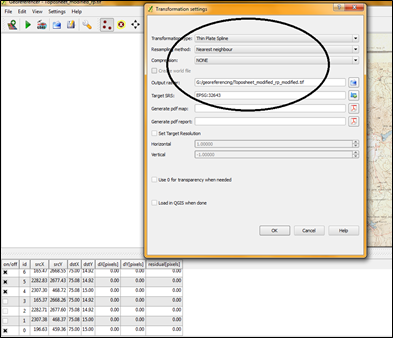
- After entering GCP’s click on Settings option in Georeferencing menu bar select Transformation Settings option. A drop box will be displayed and select options as shown in the below image. Specify output file name and transformation parameters and projection system then click OK.
- Click on File menu and Select Start Georeferncing option. The Georefrencing will be started.
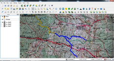
Digitising vector data
Digitising features (water bodies) of Topo map:
- Open the raster file you have geo referenced by clicking Layerà Add raster layer option.
- The raster layer window will be open and load the saved layer. It will be displayed on Map canvas.
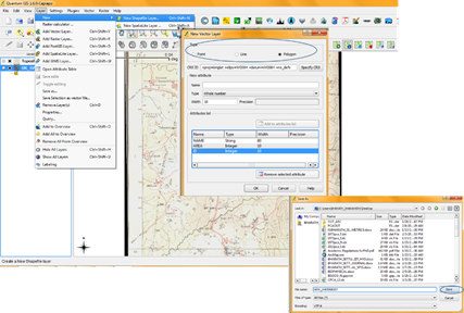
- To digitise the water bodies select Layer menu and click Newàcreate new shape file layer option. Then new shape file layer drop box will open with options.
- Select polygon option and provide the attributes for it and save the file with a name. The saved new shape file will be loaded for creation of features.
- Attributes are entered as features to be created.
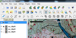
- Zoom to the feature you want to digitize by using zoom options. Right click on the vector layer you have created and select Toggle editing (pencil like symbol) option. Then tool bar will be highlighted. Click on capture polygon icon and start digitizing the water body.
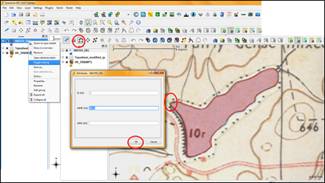
- Enter the attributes and press ok. After digitisation click save layer option to save the modifications you made.
- To compute area of the polygon right click on the layer you digitised and click open attribute table and select field calculator select area option to compute area.
- The area will be shown in degrees. Convert it to Hectares by adding new column and provide the name for new column. Then select field calculator select the new column to be updated.
- Type the formula as AREA*110*110*100 for getting in terms of Ha.
Importing Google earth data:
- To load a vector file click on Layer menu in menu bar select add vector layer, a dialogue box will be displayed, which allows to traverse through the file system and load a kml file which you have created using Google earth or other formats of vector data.
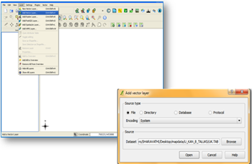
- The layer will be displayed in the map canvas area.
- Right click on the layer and select properties to check the attributes, colors etc.
- QGIS supports a number of Symbology renderers to control how vector features are displayed
- Labels tab allows to enable labelling features and control a number of options related to fonts, placement, style, alignment and buffering.
- Attributes tab allows to manipulate the attributes of the selected dataset
- General tab permits to change the display name, view/change the projection of vector
- Metadata tab contains general information about the layer which is not yet editable.
- Diagram tab used to overlay a graphics to a vector layer. It allows overlying pie charts, bar charts.
- Right click on the layer click save as option to create a shape file. Import the shape file and continue to work with it. So you can edit the features and compute the area etc.
Help from QGIS:
http://www.qgis.org/en/site/forusers/index.html#
http://www.qgis.org/en/docs/index.html
4.0 WATER YIELD IN THE CATCHMENT
Objective: To estimate the water yield in a catchment (of a lake, pond, stream or river).
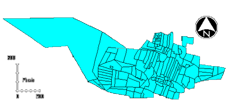
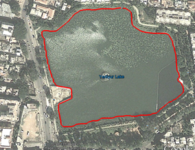
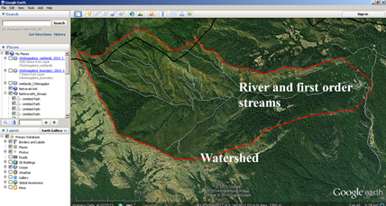
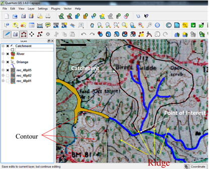
Catchment (Drainage area, Drainage Basin or Watershed): The area of land draining water into a water body (fig1). Two neighboring catchments are separated by a ridge (highest land that separates two watersheds). The areal extent of a catchment is obtained by tracing the ridge on a Topographical Map (fig2). Based on the spatial extent, catchments are classified given in table 1.
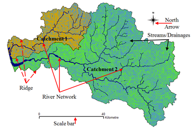
Fig1: Catchment Map
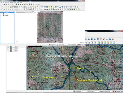
Fig2 : Topographic map indicating different features
Table1: Classification of Catchments in India
Sl.no |
Type of Catchment |
Area in 1000 Hectares |
1 |
Micro-watershed |
Less than1 |
2 |
Milli-Watershed |
1 – 10 |
3 |
Sub-Watershed |
10 – 50 |
4 |
Watersheds |
50 – 200 |
5 |
Sub-Catchments |
200 – 1000 |
6 |
Catchments |
1000 – 3000 |
7 |
Basin |
3000 – 25000 |
8 |
Region |
Greater than 25000 |
Source: http://fes.org.in/source-book/SWC%20Source%20Book_final.pdf
Contours: Contours are the imaginary lines on the earth surface with equal elevation. In a topographic map of 1:50000 scale, contours are at every 20 metre interval. Contours with decreasing altitudes with respect to an higher altitude contour indicates hillock, on the contrary increasing contours along a low altitude contour indicates Valley.
Steps involved in Delineating a Catchment:
Step 1. Scan the respective topographic map
Step 2.Use QGIS, Geo-reference or assign the co-ordinates
Step 3. Digitise waterbody as polygons and Stream network as line features.
a. Create New features as line or polygon
Go to Layers, New Shape file Select Line or Polygon feature based on the feature to be delineated, add attributes and save.
b. Load the new shape files created, click on toggle editing, click on add feature and start delineating the feature, save the edits. And stop toggle editing.
With respect to the water body, digitize its catchment as polygon feature.
step 4. Compute the spatial extent of the catchment. To measure the Area, right click on the catchment layer, click on properties, toggle editing, add column (the same procedure could be adopted to define the attribute), provide the details of the attribute such as attribute name, type such as text, integer or float and then ok. Click on the Field Calculator, click on update field and select the field to be updated (Area). Add the Area Operator to the field calculator expression to estimate the area of the polygon (Catchment). Save Edits and Stop Toggling.
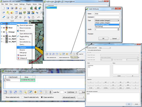
step 5. Click on the Open Attribute to obtain the information about the area estimated. [very important: if you have the coordinate system in latitude longitude degree decimal coordinate system, are would be in square degrees, if the coordinate system is UTM then the area would be as square metres. To convert square degrees to hectares multiply the area measured with 1100*1100, and to convert square metres to hectare divide area measured by 10000]. In the above example demonstrated, area is 152.5 Hectares.
Similarly, other measurements such as distance, coordinates, centroids etc. along with other vector operations could be made using Calculator TOOL.
Rainfall: Daily Rainfall data at different locations are observed using rain gauges as millimeter and maintained by India Meteorological Department (IMD), Public Works Department (PWD), Water resources Development Organisation (WRDO), Agriculture Department, Revenue Department, Forest Department, etc, and is as depicted in fig.3. Each rain gauge represents rainfall over an area assuming rainfall is uniform in its vicinity
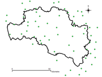
Fig 3: Rain Gauge stations
.
To analyze the rainfall trend and dynamics over a region, seasonal and annual rainfall data for atleast 10 to 20 year.
Steps involved in analyzing rainfall trend in the basin:
step 1. Rainfall data for 15 to 20 years shall be acquired from the agencies such as IMD (Indian Meteorological Department), WRDO, Statistical department etc.
step 2. Rain gauge stations inside and near to the basin are identified based on the location of the rain gauge stations.
step 3. Annual data is plotted as a graph to understand the dynamics of rainfall over time.
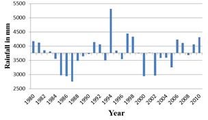
step 4. Based on the annual rainfall trend, seasonal variation in the watershed is estimated
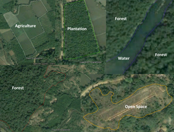
Extraction of Land use details from Google Earth: Google earth provides satellite images with high resolution, this could be used to identify different types of land uses in the basin.
Steps involved in extraction of landuse features from Google earth:
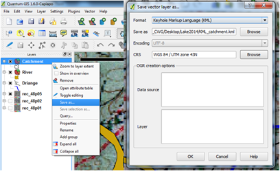
step 1. The delineated catchment would be in the form of xxx(filename).shp format i.e., as a shape file, first convert the same to kml. Right click on the shape file, click on save as, click on format and select KEYHOLE MARKUP LANGUAGE (KML) to convert the convert the file to kml, save the file
step 2. Double click on the saved ‘kml’ to open the same in Google earth
step 3. Within the watershed, start digitising layers as polygons and save as ‘kml’.
Example: Agriculture as a layer, Forest as a layer, water body as a layer etc
step 4. ‘kml’ files are imported in QGIS, and converted as shape file (same procedure as step1)
step 5. Calculate the are under each landuse using Map calculator tool
Assessment of water yield: Water yield or Surface Runoff is the precipitated water that drains to a water body in a catchment. Surface runoff occurs during monsoon. Factors affecting Runoff are the Slope, Drainage, Land use, Soil Characteristics, Rainfall. The total quantity of water that can be expected in a stream in a given period of time such as monthly, annual etc… is referred to as Runoff Yield.
Runoff Yield (Q) as kilo.cubic metre (Million Litres) is estimated empirically (eq.1) as a function of Rainfall (P) in mm and Area under different land uses (A) in Hectares.
Q = (C*P*A)/100 1
Where Q = Runoff Yield in Million litres
C = Runoff Coefficient of a particular land use
A = Area under land use in Ha
P = Mean Monthly rainfall in mm (average of 10 – 15 years)
Runoff Coefficient under different land use is as specified in table 2.
Land Use |
Runoff Coefficient |
Forests |
0.1 – 0.2 |
Plantations |
0.2 – 0.6 |
Agriculture |
0.4 – 0.7 |
Open Spaces, Grasslands |
0.5 – 0.8 |
Built-up |
0.7 – 0.9 |
Rocky Areas |
0.8 - 1.0 |
Water Yield Estimation
Location Description |
|
Catchment Extent |
Latitude |
Longitude |
min |
min |
max |
max |
Catchment Area in Ha |
|
Annual Rainfall in mm |
|
Land Use |
Area in Ha A |
Runoff Coefficient C |
Forests |
|
|
Plantations |
|
|
Agriculture |
|
|
Open Spaces, Grasslands |
|
|
Built-up |
|
|
Rocky Areas |
|
|
Monthly rainfall P in mm |
January |
February |
March |
April |
May |
June |
|
|
|
|
|
|
July |
August |
September |
October |
November |
December |
|
|
|
|
|
|
Seasonal Catchment Yield in Million Litres Q = (C*A*P)/100 |
Land Use |
January |
February |
March |
April |
May |
June |
Forests |
|
|
|
|
|
|
Plantations |
|
|
|
|
|
|
Agriculture |
|
|
|
|
|
|
Open Spaces, Grasslands |
|
|
|
|
|
|
Built-up |
|
|
|
|
|
|
Rocky Areas |
|
|
|
|
|
|
Gross Yield Q |
|
|
|
|
|
|
Land Use |
July |
August |
September |
October |
November |
December |
Forests |
|
|
|
|
|
|
Plantations |
|
|
|
|
|
|
Agriculture |
|
|
|
|
|
|
Open Spaces, Grasslands |
|
|
|
|
|
|
Built-up |
|
|
|
|
|
|
Rocky Areas |
|
|
|
|
|
|
Gross Yield Q |
|
|
|
|
|
|
Annual Catchment Yield = (Σ Q) |
Million Liters |
5.0 FLYING FRIENDS…. |
Introduction: Birds (class Aves or clade Avialae) are feathered, winged, two-legged warm-blooded, egg-laying vertebrates. Aves ranks as the tetrapod class with the most living species, approximately ten thousand. Extant birds belong to the subclass Neornithes, living worldwide and ranging in size from the 2 in Bee Hummingbird to the 9 ft Ostrich. The fossil record indicates that birds emerged within the theropod dinosaurs during the Jurassic period, around 150 million years ago. Archaeopteryx was the first fossil to display both clearly traditional reptilian characteristics: teeth, clawed fingers, and a long, lizard-like tail, as well as wings with flight feathers identical to those of modern birds. It is not considered a direct ancestor of modern birds, though it is possibly closely related to the real ancestor. Depending on the taxonomic viewpoint, the number of known living bird species varies anywhere from 9,800 to 10,050. In India, around 1314 species of birds are documented, of which 42 are endemic to India. In Karnataka state, 535 species of birds has been reported. |
Evolution: Modern birds are characterized by feathers, a beak with no teeth, the laying of hard-shelled eggs, a high metabolic rate, a four-chambered heart, and a lightweight but strong skeleton. Wings are evolved forelimbs, and most bird species can fly. Flightless birds include penguins, and diverse endemic island species. Some species of birds, particularly penguins and members of the Anatidae family, are adapted to swim. Birds also have digestive and respiratory systems that are uniquely adapted for flight. Some birds, especially corvids and parrots, are among the most intelligent animal species; several bird species make and use tools, and many social species culturally transmit knowledge across generations. |
Behaviour: Many species annually migrate great distances, and many more perform shorter irregular movements. Birds are social, communicating with visual signals, calls, and songs, and participating in such social behaviours as cooperative breeding and hunting, flocking, and mobbing of predators. |
Usefulness: They eat a lot of harmful insects that may destroy crops. they are part of the food chain. They help disperse the seeds of many plants. The raptors keep rodent populations in check. The vultures help clean the land of animal carcasses, preventing the spread of infectious diseases. Another use of birds is harvesting guano (droppings) for use as a fertilizer. Birds prominently figure throughout human culture. About 120–130 species have become extinct due to human activity since the 17th century, and hundreds more before then. |
Need to study: Birds are among the most fascinating creatures on Earth. Many are beautifully colored. Others are accomplished singers. Many of the most important discoveries about birds and how they live have been made by amateur birders. Ornithology is the scientific study of birds. The information ornithologists gather is used to better understand how birds function, inside and out, and to learn how birds relate to their natural environment.
- Birds provide a terrific doorway into nature and scientific study.
- They are easy to see and study.
- They engage in fascinating behaviors and play important roles in the ecosystems that sustain life
- Birds are excellent indicators of environmental health.
- Their changing populations often provide clues to the overall health of their habitat.
|
Requirements: A pair of binoculars, good pictorial field guide and note book to pen down observation. |
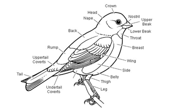
Parts of a bird
|
-
Head: The bird's head is one of the best places to look for field marks such as eye colour, malar stripes, eyebrows, eye rings, eye lines and auricular patches. The crown (top) and nape (back) are also key parts of the head that can help identify a bird.
-
Bill: The size, shape and colour of a bird's bill is critical for identification. Also check for any curvature in the bill or unique markings such as differently coloured tips or bands.
-
Chin: The chin, directly below the bill, is often hard to see on many birds, but when it is a different colour it can be an exceptional body part to check for identification.
-
Throat: A bird's throat may be a different colour from its surrounding plumage, or it may be marked with spots, streaks or lines. Malar stripes may frame the throat as well, helping set it off from the rest of a bird's body. For many birds, the chin and throat have similar colours and markings.
-
Neck: The neck of a bird is hard to see on many species, since it can be relatively short and insignificant. On wading birds, however, the neck is much more prominent and can be a good place to look for field marks. The length of the neck can also help distinguish different bird species.
-
Back: A bird's back is often broad and easy to see in the right posture. Different colours and markings along the back that distinguish it from the neck, rump and wings.
-
Chest: The chest (also called the breast) is the upright part of the bird's body between the throat and the abdomen. A bird's chest may be differently coloured or marked with stripes, streaks or spots that can help with identification.
-
Abdomen: The abdomen or belly of a bird extends from the bottom of the chest to the under-tail coverts. The colours and markings on the abdomen may vary from the chest and flanks, making it a good feature to check for identification.
-
Flanks: The flanks (sides) of a bird are located between the underside of the wings and the abdomen. In many bird species, the flanks have unique colours or markings, though depending on how the birds carry their wings, the flanks may be difficult to see.
-
Wings: Birds' wings are their upper limbs used for flight. Wing bars or patches are useful field marks, as are the lengths of the wings compared to the length of the tail when the bird is perched. In flight, wing shape is also a great field mark.
-
Rump: A bird's rump is the patch above the tail and low on the back. For many birds, the rump does not stand out, but some species show unique rump colour patches that are useful for identification.
-
Tail: The length, shape and colours of a bird's tail are important for proper identification. The tail can be held in different positions when the bird is perched or flying. Also, watching for different markings can help distinguish different birds.
-
Under-tail Coverts: The short feathers beneath the tail are the under-tail coverts, and these feathers often show unique colours or markings that can distinguish bird species.
-
Legs: Birds' legs vary in length and colour, both of which can be useful field marks for proper identification. The thickness of the leg, while difficult to see on many species, can also be a clue, as can any feathering. Some raptors, for example, have heavily feathered legs that can be used to identify the birds.
-
Feet: Many birds' feet are the same colour as their legs, but not always. The orientation of the toes, the size of the talons and how a bird uses its feet are also useful identification characteristics.
|
Field Analysis:-
Method - Random Sampling
Equipment used - Binoculars, Digital SLR Camera
Duration – every month last Sunday
Weather Conditions: Day light: Sunny/cloudy
Temperature: |
Date |
Location |
Habitat |
Birds |
comment |
|
|
|
|
|
|
|
|
|
|
|
|
|
|
|
|
|
|
|
|
|
|
|
|
|
|
|
|
|
|
|
|
|
|
|
|
|
|
|
|
|
|
|
|
|
|
|
|
|
|
|
|
|
|
|
|
|
|
|
|
|
|
|
|
|
|
|
|
|
|
|
|
|
|
|
|
|
|
|
|
|
|
|
|
|
|
|
|
|
|
|
|
|
|
|
|
|
|
|
|
|
|
|
|
|
|
|
|
|
|
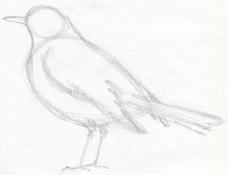
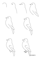
How to sketch a bird in field? |
|
|
|
|
Common Friends in Bangalore |
|
 |
 |
|
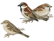
House Sparrow (Passer domesticus) |
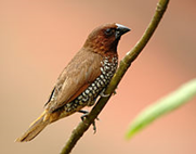
Spotted Munia (Lonchura punctulata) |
|
 |
 |
|
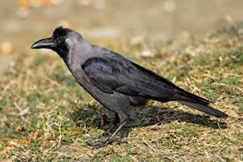
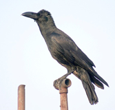
House Crow (Corvus splendens) |
Jungle Crow (Corvus macrorhynchos) |
|
 |
 |
|
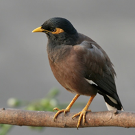
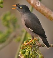
Common Myna (Acridotheres tristis) |
Jungle Myna (Acridotheres fuscus) |
|
 |
 |
|
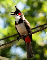
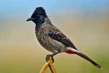
Red-whiskered Bulbul (Pycnonotus jocosus) |
Red-vented Bulbul (Pycnonotus cafer) |
|
|
|
|
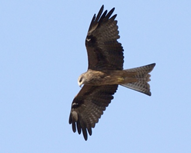
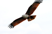
Black Kite (Milvus migrans) |
Brahminy Kite (Haliastur indus) |
|
|
|
|
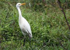
Cattle Egret (Bubulcus ibis) |
Rose-ringed Parakeet (Psittacula krameri) |
|
|
|
|
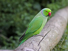
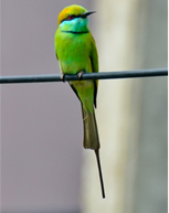
Green Bee-eater (Merops orientalis) |
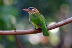
White-cheeked Barbet (Megalaima viridis) |
|
6.0 GEOTAGGING AND FIELD DATA COLLECTION
Geotagging: Geotagging (is the process of adding geographical identification metadata to various media such as a geotagged photograph or video, websites, SMS messages. This data usually consists of latitude and longitude coordinates, altitude, distance, accuracy data, and place names.
Geotagging photographs is the process of recording location information (the latitude and longitude) where and when a photograph was captured by the camera. The data is recorded within the digital image file that the camera records and this data can be read by any suitable software.
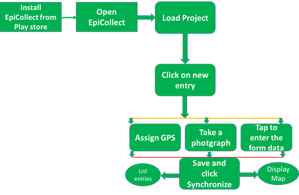
STEPS INVOLVED IN GEOTAGING AND FIELD DATA COLLECTION:
Go to play store in your Android mobiles
Search for EpiCollect software, download and install it.
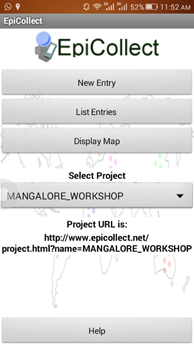
Open EpiCollect application and the welcome screen is
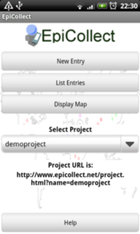
By default, demo project will be loaded.
To load a new project, select Menu option and load project
Load “MANGLAORE_WORKSHOP” Project, which is created to geo-tag plants:
Click on New entry,

Click on assign GPS to get location (x, y: longitude, latitude) details. It takes some time for assigning GPS. You need to wait for few seconds for good accuracy.
Tap to take a photograph for capturing new photo of a sapling. If you have already saved the photograph, you can upload the same). Take a photograph and click save.
Tap to enter form data
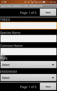
After entering press confirm button and press Tap to synchronize to server.

You can also list the earlier data you have entered in List entries section
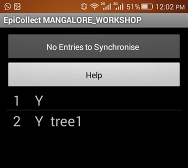
Click on one entry and preview the entry.
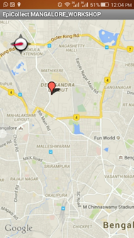
Click on View on Map to visualize on Google maps backdrop.
A simple flow chart of working with EpiCollect
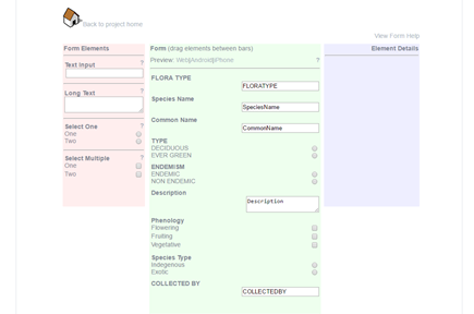
You can create your own project at http://www.epicollect.net/create1.html by providing a new name for your project.

Add the fields which you required for the collection of data input it and save the form.
ANOTHER SIMPLE SOFTWARE FOR FIELD DATA COLLECTION
- Install “MAPinr-KML/KMZ/WMS/GPX/OFFLINE” from Google Play Store -For Android users. MAPinr is a simple and free Android app that allows you to manage your kml/kmz/gpx files and view them on different maps.
- In your phone switch on GPS shortcut button.
- Open Mapinr app and you will get welcome screen.

- Click on menu option select new file and provide file name.
- Click on back drop map to be displayed. Select the option of OSM to Google maps, which ever required.
- Go to settings select auto save option to save the session for without losing the information.
- Clock on map Waypoint option to record GPS location. Then the Latitude and Longitude will be displayed as
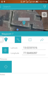
- Then if you want to take picture click + symbol to add pictures and save it.
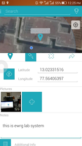
- You can enter Attribute data corresponding to the waypoint location in the note section.
- Time stamp will be stored your time of location point recorded.
- If you want, you can change the pin color, symbol etc.

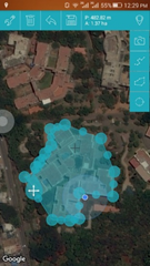
- If you want to measure length and area you can do it with options selecting poly line and polygon symbol available in home screen as shown.
- If you want to change the measuring units go to Setting and change it.
- If you have already created some data in the form of KML file you can import and visualize here.
- You can share the file with your friend by clicking Share option in the Menu bar. You have options suc
- has Shareit; Bluetooth; Mail; Gmail and you can send it to Google drive.

7. Pollen study and its application – a brief overview
Pollination, the life supporting function of plant world, is considered as one of the most valuable ecosystem services as per human assessment (Mburu et al. 2006). Pollination is defined as “ the process of moving pollen from the anthers of one flower to the stigma of another or the same flower”(www.fao.org). This simple transfer of pollen grains to ovule and subsequent chain of events have led to quests on evolution, biodiversity, species-species interaction and economic prospects. Considering only the economic importance of pollination, an estimation of £153 billion per annum has been calculated at global level (Breeze et al. 2011). Apart from bee the major pollinator, pollination is usually mediated through beetles, bugs, butterflies, moth, flies, birds even through large animals like humans too. The focal point of pollination is successful transfer of pollen grains to flower’s receptive surface i.e. stigma. Depending on destination pollination can be classified as self (within same flower) and cross (to other flower). Similarly, based on mode of pollen transfer it can be anemophily (wind mediated), zoophily (animal mediated) or hydrophily (water mediated).
Pollen: Morphology, development and function
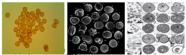
Pollen, the pivotal component of pollination mechanism deserves attention in this regard. Apart from its role in pollination it has many use in other disciplines, both academic and commercial aspects. Pollen, at a glance can be characterized as haploid, small in size, resistant to decay and enormous in production. Morphologically, pollen can be of many shapes, round, pyramidal, elliptical, square and intermediate variations. The cell has two layers, outer layer, exine and inner layer intine. It is the exine which helps most in pollen identification and survival. Exine has sporopolenin, the protein which is responsible for pollen’s extraordinary survival power against desiccation. Exine is also decorated with pores and slits, accordingly pollen can be classified as porate (with pores) and colpate (with slits). In addition to that, many a times exine has additional ornamentations (spine, network etc.) which also helps in classification.
transmission electron microscope (TEM)
Pollens are present inside the anthers. They are generated from pollen mother cell (P.M.C) through meiosis. Initially, the resultant cells from meiosis form a tetrad which later on dissociates into single pollen grain. During fertilization, pollen cell gives rise to two sperm cells, among which one fixes with ovule forming diploid zygote and another one joins with central cell to form tri-nucleate endosperm.
Pollen study methods– Pollen study is a part of Palynology, where plant pollen along with spores and microscopic planktonic organisms are studied in both living and fossil form.
A typical study plan includes following steps –
a) selection of study area (based on objectives): Forest, open land, lakes, mines, ancient sites / objects, air (practically any space can be selected)
b) collection of pollen: Pollen collection should be done under sterile condition (as much as possible). There is always chance of contamination through wind, surrounding material, animals, human interaction and even sampling items. Therefore, collection process should be fast, preferably clean and collected material must have proper labelling. For surface collection of sample, a spoonful of sediment (with replica) is enough for serving the purpose (the amount can vary also. For stratigraphic column, collecting samples at 2 cm vertical intervals ( 1cm3 – 20cm3 ) is mostly recommended (Cummings 2007). For air borne pollens, pollen samplers are used for collection.
c) processing of sample: Collected samples can be stored under refrigeration until laboratory work begins. Pollen processing is mostly chemical based with an aim to remove all debris attached with the particle. Standard procedure is as follows –
Incubation with 10% hydrochloric acid (HCl) for overnight (for calcium carbonate removal)
Addition of sodium polytungstate for density separation
Separation of organic layer through centrifugation
Addition of acetolysis mixture (9:1, acetic anhydride : sulphuric acid) to remove non-pollen organogenic material
Centrifugation and sequential wash with glacial acetic acid and distilled water
Ethanol addition for precipitation
Removal of ethanol and addition of glycerol for mounting
Preparation of slide and counting
d) pollen counting: Pollen count can be done under light microscope and observed grains should be compared with reference collection from the related area. In ideal circumstances, at least 300 pollen grains would have been counted, however it depends on concentration of grain recovered after processing.
Palynoassemblage recovered from the surface samples (source: Tripathi et al., 2016, DOI:10.1080/01916122.2015.1045049)
e) observation and deduction: At first glance, pollen slides provide information on pollen morphology, and their variation in a given study area. For surface sample studies combination of slides from different sample sites provide an overall view of the pollen profile from the study area. This pollen profile/diagram can be compared with the vegetation information available from the region.
For stratigraphic studies, pollen profiles from different depths depict the changing vegetation patterns taken place in temporal scale. By radiocarbon dating, it is possible to detect the age of the different strata which then can correlate with available pollen variation. The pollen profile/diagram developed from this study has major contribution in paleovegetation/paleoclimate reconstruction.
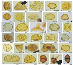
Palynoassemblage recovered from the surface samples (source: Tripathi et al., 2016, DOI:10.1080/01916122.2015.1045049)
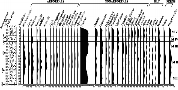
Past vegetation structure-Pollen diagram from sedimentary sequence of Bargarh District, Odisha
Tripathi et al. 2014, DOI: 10.1016/j.quaint.2013.12.005
Application of pollen study – Pollen study has multiple applications, which can be broadly categorized into two groups, though many times they are interrelated.
Academic work / integration in other discipline – Paleobiology – the most notable use is in paleobotany to understand past vegetation composition and distribution. Identification of fossil pollen and its affinity with present members would be helpful for evolutionary biology, phylogenetics and addressing issues related to land plant evolution, paleoclimate reconstruction and archeobotany.
Pollen study shed light on human-nature interaction in various ways, like ancient diet construction, crop domestication, crop introduction and social and cultural activities etc.
Geology – pollen composition and form at different sedimentary strata provides detail input related to sedimentation process, prevailing temperature and fossilization output.
Industrial / practical use –
Oil and gas exploration – As oil and gas (“fossil fuel”) originating from vegetation, pollen presence in stratigraphic layers is used as indicator of fossil fuel presence. It is the pollen abundance / density, diversity and coluring pattern which are determinants of fossil fuels presence and quality.
Melissopalynology – One of the interesting use of palynology is in product authentication eg. Honey. Honey has an estimated world production of 3.6 billion pounds in 2011 and the product can be broadly categorized into general and custom made (Phipps 2014). General honey which has more wide circulation network often falls prey to manufacturers false claim of genuineness. The thorough screening of unprocessed honey which most often has trace amount of pollen provides information on source of honey/parent tree, area/country of origin, detection of adulterant, antibiotics etc. On the other hand, custom made honey eg. organic/certified honey, particular tree based honey as per customers’ choice of preference which has niche market but high demand, is very much dependent on authentication which determines their market share.
Museology – Pollen study provides support to authenticate genuineness of the antique pictures/artefacts to some extent. Paintings especially which have been done in outdoor setup, often have captured pollens in the canvas which could provide information on location and season of the painting, source of the material etc. By corroborating pollen study result with associated information the genuineness or artist/agents’ claim can be validated.
Custom / Excise application – detection of narcotics, their country of origin, possible route of travel even media of transport can be identified and spotted through pollen analysis.
Forensic science – The successful application of pollen study in crime solving scenario is perhaps most widely referred examples of palynology application. Pollen prints’ detection over victim’s/suspect’s body or any other crime scene objects is an indicator of crime area identification, tracing identity and motive of the crime.
Healthcare – seasonal release of pollen grains, their identity and abundance are useful for making pollen calendar. These calendars are prerequisite for any clinical technicians and medical professionals for treating air borne allergy cases.
8.0 MANGROVES
Most mangroves are woody plants, shrubs and trees. There are also few herbs, mainly some grasses and sedges. Among the woody plants one is a lower plant- a fern namely Acrostichum aureum this fern grows in colonies in swampy and marshy places where the tidal force is low and salinity is not that high.
I. TRUE MANGROVES
Family: Rhizophoraceae - This is the most important family of mangroves. The members are woody plants, usually trees. The family has spectacular development of aerial stilt roots. These roots spring from the main stem and also the branches; they branch repeatedly and grow downwards and give additional support to the tree in the soft mud. The aerial roots, studded with tiny air passing windows known as lenticels, visible to the naked eye, also help in aeration.
The trees have opposite, simple, dark green leathery leaves. The terminal bud is protected by a long cover made up of stipules. These stipules fall off when new leaves emerge. The members of the family produce from the fruits long, green, cylindrical propagules. These on maturity detach from the fruit and fall vertically into the mud, where they strike roots and become daughter plants. If the propagules happen to fall when the substratum is flooded during high tides they may be carried away by water currents; On reaching suitable swampy places they develop into new plants. This interesting phenomenon of reproduction is called ‘vivipary’. Here apparently the mother plant is giving birth to daughter plants.
Members of Rhizophoraceae can be identified using the following key:
Calyx 8-16 lobed; petals 2 lobed : 1. Bruguiera
Calyx 4-6 lobed; petals not lobed:
Calyx 4 lobed; petals without apical outgrowths : 2. Rhizophora
Calyx 5-lobed; petals with apical outgrowths;
Stamens more than 12 : 3. Kandelia
- Bruguiera: It is a tree with rough corky bark; stem base may be flattened into buttresses. Leaves elliptic to oblong elliptic with a narrow tip; but not ending in a narrow long point as in Rhizophora. Leaf size 7-14 cm by 4 to 6 cm. Leaf stalks and midrib red coloured. Flowers in singles, reddish coloured; calyx 10-16 lobed, red to pinkish; petals bilobed, outer margin with silky hairs. The fruit produces a propagule of 10-15 cm. which is slightly angled. Small trees were found at Hegle in Venktapur river of Bhatkal. In Andamans it grows to 36 m, and is buttressed.
2. Rhizophora:
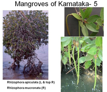
R. mucronata: Trees reaching maximum height of 10 m in the Division. Numerous branched stilt roots arise from the base of the stem. Some arise from the branches also. Leaves 10-18 cm X 4-10 cm, broad and elliptic; the leaf tip is produced into a narrow outgrowth called mucro; leaf base blunt to obtuse. Flowers are produced in long clusters, each cluster having 4-8 flowers. Petals are hairy and stamens 8. The propagule, a long green, smooth cylindrical structure, reaches a maximum length of 65 cm .
Note: Both Rhizophora mucronata and R. apiculata are found in Honnavar Division. The former is the commoner and widely used for afforestation.
R. apiculata: A smaller tree, reaching 4-5 m in the Division. Stilt roots arising from main stem as well as from branches form impenetrable barrier beneath the canopy. Leaves elliptic lanceolate with a smaller narrow bristle like point towards the narrow tip. Size 10-20 cm X 5-8 cm. Leaf base conical; leaf middle vein reddish. Flowers in pairs in upper leaf axils, without stalks; petals not hairy; stamens 12. Propagules 30-50 cm long .
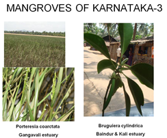
3. Kandelia candel: Small trees reaching 5-6 m high. Leaves narrower than Rhizophora, oblong shaped. Flowers white, in dichotomously branched inflorescence axis. Calyx 5 lobed, reflexed; petals 5, divided into numerous fine branches. Stamens numerous. Propagule cylindrical, green, narrowed towards the tip, 30-40 cm long. The trees have flesh coloured base flattened into buttresses; stilt roots closely adpressed to the stem base. Bark reddish brown, peeling off into flakes
Note: Found commonly in all estuaries
Family: Sonneratiaceae - Buttresses absent; pneumatophores (breathing roots) corky and soft, rising vertically into the air from the mud. Leaves opposite, simple; flowers large with numerous free stamens.
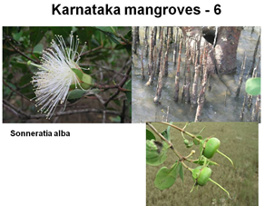
Sonneratia alba: Small trees reaching maximum of 5 m. Many corky pneumatophores stick out of the mud from all around the tree. Leaves opposite, elliptic, oblong, blunt at apex, narrowed at base; Flowers 2-3 together; calyx has a cup shaped part and 6-8 lobes which are distinct in fruit. Petals white, small; stamens numerous, free, white; ovary depressed globose. Fruit somewhat spherical, many seeded with calyx remaining in the fruit. Natural regeneration is plentiful especially in shallow places with low tidal effects .
Note: Found in all rivers except Sharavathi
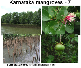
Sonneratia caseolaris: Trees up to 12 m height; soft corky pneumatophores longer than S. alba, reaching up to 1 m. Young stem 4-angled. Leaves almost without stalk, much narrowed at base, opposite. Leaf tip has a pore known as hydathode through which excess salt is secreted. Flowers reddish purple, in singles at the tip of branches; stamens numerous, reddish. Fruits depressed globose
Note: Most common mangrove tree in Sharavathi; Rare in other rivers; not found in Gnagavali, although Rao & Suresh (2001) present it as a cpmmon species there. It prefers places with low salinity; the Sharavathi river, where fresh water from the dams is constantly released appears to be ideal for it.
Family: Avicenniaceae - Shrubs or trees without buttresses. Breathing roots (pneumatophores) numerous and protruding from the mud all around the tree. Leaves opposite, without stipules; flowers yellow. Fruit one seeded, dry when mature.
Avicennia marina: Shrubs or small trees upto 4 m high. Bark smooth yellowish brown. Leaves 3-6 X 2.2.5 cm, elliptic oblong or ovate, narrowing to an acute tip; leaf base rounded or narrowing. Flowers small, stalkless, yellowish clustered towards tips of floral axis; stamens not projecting out from the corolla. Fruit at maturity ovoid with a pointed tip, slightly flattened .
Note: Very common in Gangavali, rare in Aghanashini, common in Alvekodi creek, absent in Sharavathi and Badgani, moderate in Venktapur.
Avicennia officinalis: Larger trees, reaches 8-10 meters in Honavar Forest Division; exceptional individuals of 12 m are found in the sacred grove of Masurkurve in Aghanashini. Smooth whitish gray bark; pneuatophores seen all around the tree. In addition masses of branching stilt roots hang from the upper part of the trunk and base of large branches. Leaves 5-7.5 cm X 2.5- 3.25 cm, ovate, oblong with more or less rounded leaf tip. Small, yellow stalkless flowers seen in clusters towards the tip of floral axis. Flowers distinguished from A. marina by stamens seen projecting outside the corolla
Note: Found in all the rivers of the Division.
Family: Myrsinaceae - Plants without pneumatophores; flowers with 4 sepals and 4 petals; and superior ovary.
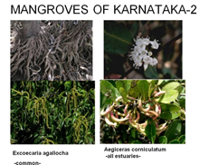
Aegiceras corniculatum: Shrubs or small trees with slender stilt roots. Leaves 4-8 cm X 2-4 cm, alternate, ovate-oblong or obovate, may have a small notch at the blunt tip; leaf base cone like. Flowers small, white, fragrant in umbellate bunches. Propagules which come out of the fruits are 3-4 cm long and curved with pointed tips .
Notes: Found in all estuaries along edges and banks away from strong tides; notable for fragrant white flowers
Euphorbiaceae - Plants with latex. Male and female flowers in separate clusters
Excoecaria agallocha:Large shrubs or small trees occurring along the edges of the swamp, on bunds and on wet soils. Acrid, blister causing latex present. Numerous serpentine roots produced from base of stem. Leaves alternate, margins entire or mostly minutely toothed; leaves turn red before shedding .
Acanthaceae - Family of herbs and shrubs. Flowers not regular in shape.
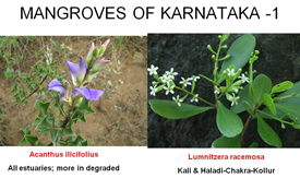
Acanthus ilicifolius: A shrubby plant growing in colonies in shallow parts of the swamp. Leaves opposite, stiff, wavy and with sharp spines along the margin. Flowers large, blue
Poaceae - The members are grasses. In the estuaries these grasses are found often forming meadows submerged during high tides and exposed during low tides.
Porteresia coarctata: A stiff erect grass growing in meadows in open shallow parts of the estuaries
II. MANGROVE ASSOCIATES
Numerous species of plants occur in association with the mangroves. These are not obligate mangroves and higher salinity is not often a prerequisite for their growth. They may also be often associated with inland habitats. These plants have certain degree of salinity tolerance. They often grow along the margins of swamps, or on estuarine bunds. Details of notable mangrove associates are found in Table 2.1.
Table 2.1. Details of notable mangrove associate species in Honavar Forest Division
Sn |
Name |
Family |
Remarks |
1 |
Cerbera manghas
(Kan: Cande)
|
Apocynaceae |
Shrub or small tree with white latex and white flowers and mango sized green fruits; old fruits fibrous |
2 |
Barringtonia racemosa
(Kan: Samudraphala) |
Barringtoniaceae |
Small to medium tree with 15-30 cm long leaves, and pink flowers in long hanging inflorescences. |
3 |
Dolichandron spathacea |
Biganoniaceae |
Tree close to coastal swamps with white fragrant flowers, and long bean like compressed cylindrical pods |
4 |
Capparis spp.
|
Capparidaceae |
Spiny climber on bunds |
5 |
Crateva magna
|
Capparidaceae |
Small trees on the bank of Aghanashini near NH bridge; leaves 3 foliate; yellowish flowers with hard fruit. |
6 |
Calophyllum inophyllum
(Kan: Honne) |
Clusiaceae |
Large evergreen tree; white fragrant flowers and greenish yellow ripe fruits with a single seed. |
7 |
Cyperus malaccensis |
Cyperaceae |
Grass; abundant in Sharavathi backwaters. |
8 |
Diospyros embryopteris |
Ebenaceae |
Small evergreen tree with guava sized gummy fruits. |
9 |
Bridelia scandens |
Euphorbiaceae |
Climbing shrub with greenish yellow flowers small bluish-black fruits. |
10 |
Acacia farnesiana
(Kan: Kasturijali) |
Fabaceae |
Thorny bush or small tree; leaves with minute leaflets; flowers yellow, fragrant.; pod dull brown & inflated. |
11 |
Acacia nilotica |
Fabaceae |
Small trees, rare on the coast; leaflets small; flowers golden yellow in globose heads. |
12 |
Caesalpinia bonducella
(Kan: Gajagakai) |
Fabaceae |
Climber with curved sharp prickles; compound leaves; yellow fragrant flowers; dark brown dry pod 1-2 seeded. |
13 |
Caesalpinia crista |
Fabaceae |
Large woody climber; stem and leaves with sharp curved prickles; flowers fragrant, yellow; pod one seeded. |
14 |
Derris scandens
(Kan: Handiballi) |
Fabaceae |
Woody climber with rosy flowers |
15 |
Derris trifoliate |
Fabaceae |
Woody climber common on the coast |
16 |
Erythrina variegata (Indian coral tree; Kan: Varjipe) |
Fabaceae |
Soft & light wooded tree, branches covered with small black prickles; leaves with 3 foliage; coral coloured flowers. |
17 |
Pongamia pinnata
(Kan: Honge) |
Fabaceae |
Medium sized tree with compressed pods, growing often near water courses, sea beaches and rarely on estuarine banks. |
18 |
Prosopis juliflora |
Fabaceae |
Shrub or small trees with drought resistance. |
19 |
Hibiscus tiliaceous |
Malvaceae |
Shrub or small tree with yellow flowers changing to pink in the evening. |
20 |
Thespesia populnea (Kan: Hoovarase) |
Malvaceae |
A medium sized coastal tree with heart shaped leaves on long stalks and yellow flowers resembling cotton flowers. |
21 |
Ficus racemosa
(Kan: Atti) |
Moraceae |
Tree with milky latex and hollow, edible, fleshy false fruits. |
22 |
Morinda citrifolia
(Kan: Ainshe, Tagase) |
Rubiaceae |
Small tree with large leaves, dense heads of white flowers and glossy green fruit, white when ripe. |
23 |
Pandanus fascicularis
(Kan: Ketaki) |
Pandanaceae |
A palm-like, but branched shrub with narrow very long spinous leaves with small flowers on dense axis covered with white or light yellow, very fragrant bracts |
24 |
Cynodon dactylon |
Poaceae |
Karki grass forming meadows in open shallow part of estuaries |
25 |
Sporobolus virginicus |
Poaceae |
Grass; perennial grass with good sand-binding properties. |
26 |
Salvadora persica
(Tooth-brush tree; Kan: Gonimara) |
Salvadoraceae |
Much branched shrub or small tree; rare along the bunds of Aghanashini; small round fruits dark red when ripe. |
27 |
Clerodendrum inerme |
Verbenaceae |
Shrub with white flowers |
28 |
Odina wodier
(Kan: Gojal) |
Verbenaceae |
Medium sized deciduous tree with minute flowers in panicles and small, reddish, compressed fruits with one seed. |
29 |
Premna corymbosa |
Verbenaceae |
Shrub |
30 |
Vitex negundo
(Kan: Lakkigida; Nokki) |
Verbenaceae |
Shrubs, young stem 4-angled; aromatic; leaves 3-5 foliate; terminal leaflet longer |
32 |
Vitex trifolia |
Verbenaceae |
Shrubs, young stem 4-angled; leaves 3-foliate; leaflest without stalks |
MANGROVES OF ESTUARY
Citation: Ramachandra T V, Subash Chandran M D, Bharath Settur, Deepthi Hebbale, Prakash Mesta, Rajasri Ray, Sudarshan P. Bhat, Asulabha K S, Sincy Varghese, Durga Madhab Mahapatra, Harish R. Bhat, Vinay S,. Vishnu D Mukri,,Gouri Kulkarni, Bharath H. Aithal, 2016. My Village Biodiversity: Documentation of Western Ghats Biodiversity through Network of Students and Teachers, Sahyadri Conservation Series 61, ENVIS Technical Report 113, Environmental Information System, CES, Indian Institute of Science, Bangalore 560012