| Sahyadri Conservation Series - 61 |
ENVIS Technical Report: 113, August 2016 |
 |
My Village Biodiversity: Documentation of Western Ghats
Biodiversity through Network of Students and Teachers
| 
|
| T.V. Ramachandra* |
M D Subash Chandran |
Bharath Settur. |
Deepthi Hebbale |
Prakash Mesta |
Rajasri Ray |
Sudarshan P. Bhat |
Asulabha K S |
| Sincy Varghese |
Durga Madhab Mahapatra |
Harish R. Bhat |
Vinay S. |
Vishnu D. Mukri |
Gouri Kulkarni |
Bharath H. Aithal |
The Ministry of Science and Technology, Government of India,
The Ministry of Environment, Forests & Climate Change, Government of India
Indian Institute of Science, Bangalore 560012,
*Corresponding author: cestvr@ces.iisc.ac.in,
energy@ces.iisc.ac.in
|
|
SECTION 5 : MONITERING CRABS
9.0 Monitoring CRABS
Crabs belonging to the infra order Brachyura are considered to be highly successful group of Decapoda, adapted to diverse kinds of estuarine habitats. The brachyurans form very conspicuous and bio-ecologically very important faunal constituents in estuarine ecosystem and belong to different families. The brachyuran crabs play a significant role in the coastal and marine food chains and ecology as their larvae are consumed by many predators and omnivorous fishes; they have certain check on mangrove saplings.
Morphological characteristics of Crab: The Brachyuran crabs have a depressed carapace or cephalothorax and a much reduced, straight, and symmetrical abdomen which is closely bent under the cephalothorax; this abdomen is never used for swimming and lacks biramous uropods; in the female, during the spawning season, the eggs are attached to the abdominal appendages (berried crabs).The cephalothorax has 5 pairs of walking legs, the first of which is chelate (ending in pincers) and nearly always much stronger than the other legs.
Antero-lateral teeth: The teeth of the anterolateral margins of the carapace (also called as apibranchial teeth). In some crabs anterolateral margin is smooth absence of teeth. The first anterolateral tooth is commonly called the “external orbital tooth’’ and sometime it is counted separately from the following anterolateral teeth.
Frontal margin (or front): Front is sometimes elongate, spiny form and serrated. In some crabs front is modified in to a rostrum(eg, spider crab).
The mouthparts:There are 6 pairs of feeding appendages present in mouthpart as explained below.
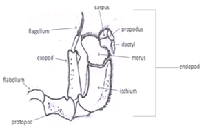
Third maxillipeds: Outer appendage of mouth part. Look at the crab en face, the third maxillipeds cover the mouth field (Fig 4). They are the appendages together they resemble a pair of doors protecting the mouth field and hiding the other mouthparts. It is attached to the body by its protopod. The endopod has distal three articles form a small palp. The endopod is composed of the large proximal ischium followed by the merus, carpus, propodus, and dactyl. The exopod consists of a long, narrow basal article and a multiarticulate flagellum. At the lateral corner of the protopod has a long setose flabellum extending through the inhalant aperture into the branchial chamber.The flabellum is used to clean the gills.
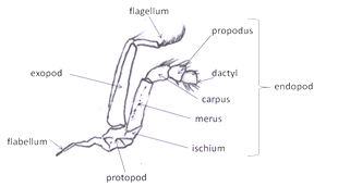
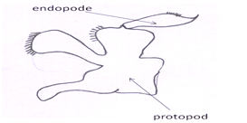
Second maxillipeds: Present underneath the third maxillipeds(Figs 5). Like the third, they bear endopods, exopods, and lateral flabellae.
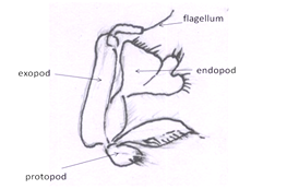
First maxillipeds: Are located, normally covered by the third maxillipeds(Fig 6).
Two smaller feeding appendages are situated below the 3 pairs of maxillipeds:
Second maxilla (or maxillules):The posterior most head appendage is the second maxilla (Fig 7) lying immediately anterior to the first maxilliped. It is small, complex, and more delicate than the maxillipeds.
First maxilla (or maxilla): The first maxilla (Fig 8)is smaller and more delicate than the second. It has two endites and an end pod but no exopod.
Mandibles: Last pair of mouthpart pair of well-calcified, jaw-like, and highly modified appendage. Anterior to the first maxillae are the large, hard mandibles (Fig 9). Each mandible consists of a heavily calcified. protopod from which arises a small palp. Only the smooth, white cutting surfaces can be seen externally.They rotate on two movable articulations, or condyles, with the head skeleton and are adapted for cutting, rather than grinding food
Antennae: Two pairs of antennae are small and may go unnoticed if they are folded out of sight under the anterior edge of the carapace (Fig 1).
Eyestalks: The two short, thick eyestalks, which are not segmental appendages, are located on the anterior edge of the head in the orbits (Fig 1). A large compound eye, located at the end of each eyestalk is composed of hundreds of independent photoreceptive units.
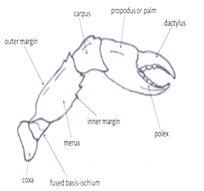
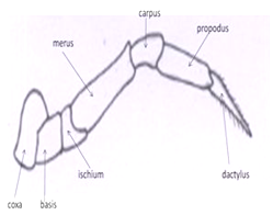
Locomotory appendages: The 5 pairs of locomotory appendages of a crab also called as the “pereiopods’’. Pereiopods includes a pair of powerful chelipeds (legs carrying a chela or pincer) and 4 pairs of walkinglegs. Pereiopode have different types of parts i.e. coxa, basis, ischium, merus, carpus, propodus and dactylus. In cheliped basis and ischium is fused. The chela itself consists of a palm (or manus) and 2 fingers, outer one of which is movable (the dactylus or movable finger), whereas the other one immovable is pollex. The tips or edges of the both fingers may be pectinated (teeth like structures).
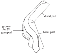
Male and female crabs are easily distinguished by the shape of their abdomen. In males, the abdomen is triangular to broadly T-shaped, whereas in females it is broad, usually semicircular, often covering most part of the ventral surface (Fig 12). Many crab species show a sexual dimorphism, with the males usually being larger or possessing special or excessively developed structures. In some species, however, it is the female which grows larger. Males possess 2 pairs of gonopods (Fig 10 & 11), that is, modified pleopods (abdominal appendages) specifically adapted for copulation most crabs practice internal fertilization. The pleopods of females are branched, setose and serve to carry the eggs fertilized eggs are exuded, attached to the setose pleopods of females, and kept there for several weeks until the planktonic larvae hatch out. Many species of crabs possess pubescence to varying degrees on their body and appendages. The hair (or more appropriately called setae) may be soft or stiff, simple or plumose (plume-like), or so short that it becomes pile-like, sometimes even short and dense, giving a velvet-like appearance. The setae may sometimes be hard and spine-like, especially on the propodus and dactylus of legs. Unlike real spines, however, those stiff setae are never calcareous. Most of the softer setae on the legs and chelae have a sensory function.
Classification of brachyuran crabs
Phylum: Arthropoda (Jointed legs)
Subphylum: Mandibulata (Having mandibles)
Class: Crustacea (Hard exoskeliton)
Subclas: Malacostraca (Biramous or branched appendages)
Series: Eumalacostraca (True soft shell)
Super Order: Eucarida (Carapace large, fused to and covering entire thorax)
Order: Decapoda (Ten legs)
Infra order: Brachyura ( having a reduced abdomenfolded against the ventral surface)
(source: http://www.niobioinformatics.in/crab/crabs/tex1.html)
General morphology of brachyuran crab
![]](s1.png)
Fig 1: Dorsal view of the brachyuran crab
|
|
Fig 2: Cheliped |
Fig 3: Walking leg |
 |
|
Fig 4: Third maxilliped |
Fig 5: Second maxilliped |
 |
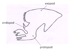 |
Fig 6: First maxilliped |
Fig 7: Second maxilla |
 |
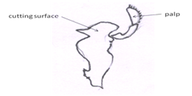 |
Fig 8: First maxilla |
Fig 9: Mandible |
 |
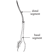 |
Fig 10: first gonopod |
Fig 11: second gonopod |
(Source: Kent E. Carpenter and Volker H. Niem 1998; FAO Species identification guide for fishery purposes, the living marine resources of the western central pacific; volume 2; ISSN1020-6868) |
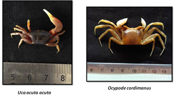
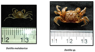
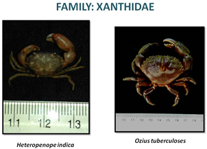
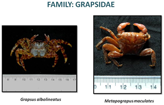
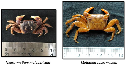
CRABS OF ESTUARY
«  »
Inventorying and mapping of Macroalgae
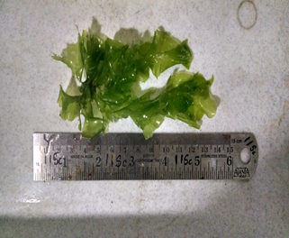
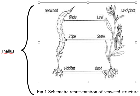
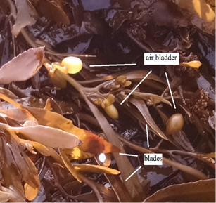
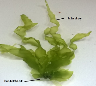
Macroscopic, multicellular marine algae or commonly referred as Seaweeds. They are of different types based on the presence of photosynthetic pigments and are categorized their colour as red, green and brown algae. Like the land plants, seaweeds contain photosynthetic pigments and with the help of sunlight and nutrient present in the seawater, they photosynthesize and produce food. Seaweeds are found in the coastal region between high tide to low tide and in the sub-tidal region up to a depth where photosynthetic light is available. Seaweeds are similar in form with the higher vascular plants but the structure and function of the parts significantly differ from the higher plants. Seaweeds do not have true roots, stem or leaves and whole body of the plant is called thallus that consists of the holdfast, stipe and blade.
-
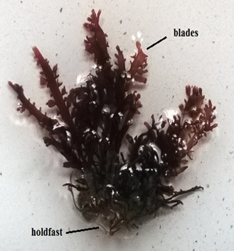
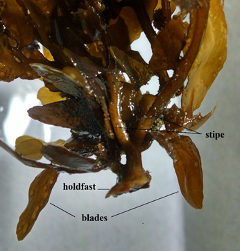
Blades: Leaf like structure which occurs in different shapes such as flattened, tubular, round, smooth, perforated, segmented, dented, etc.
-
Stipe: Stipe is the elongated stalk of seaweed which supports the blade and keep them erect
-
Holdfast or Haptera: These are structures used to attach seaweeds to hard substratum. They can be discoidal, rhizoidal, bulbous or branched depending on the substratum it attaches.
-
Float: These are structures observed in brown algae, a balloon like structure that keeps the algae afloat in the water.
Materials required for seaweed collection:
- Tide chart (http://www.tides4fishing.com/as/india/mangalore )
- Polyethylene bags
- Knife or scalpel
- Labeling materials (pen/pencil, labels, marker pens etc.)
- Rubber bands
- Field note book
Procedure:
- Reading the tide chart and marking the low tide timings and date, preferably below 1m tide should be chosen
- Samples can be selected at random as per requirement by selecting sampling points in the area
- Using the identification key below, identify the seaweed species.
- If the identification cannot be carried out in the field, sample can be carried in a zip lock cover to the lab and identified at lab using the identification keys.
- Wet preservation of seaweed samples can be done using 5-10% formaldehyde in seawater.
- Photograph of seaweeds in natural habitat can be documented as well.
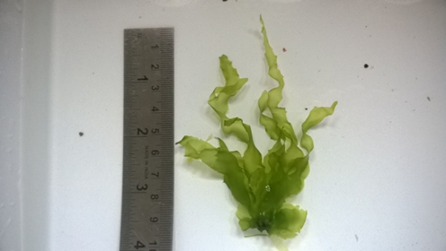
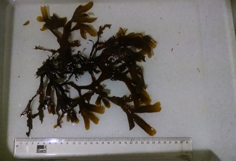
- Once the seaweeds are cleaned of all the epiphytes, dry the seaweed using a tissue and in a tray spread out the seaweed (along with a scale) and photograph.
Data compilation - Macroalgae
Name of the collector : |
Date:
Time:
Low tide (m): |
Sl.no. |
Latitude |
Longitude |
Seaweed species |
Division (Red, Green, Brown) |
Habitat (Intertidal, Supratidal, Subtidal) |
Growth Type
(Sparse, Patchy Tuft, Foliose, abundant) |
|
|
|
|
|
|
|
|
|
|
|
|
|
|
|
|
|
|
|
|
|
|
|
|
|
|
|
|
|
|
|
|
|
|
|
|
|
|
|
|
|
|
|
|
|
|
|
|
|
|
|
|
|
|
|
|
|
|
|
|
|
|
|
Fig 2. Different structures represented in all Red ,Green and Brown seaweed |
 |
 |
 |
 |
Ulva lactuca Linnaeus,1753 |
 |
|
Kingdom |
Plantae |
Phylum |
Chlorophyta |
Class |
Ulvophyceae |
Order |
Ulvales |
Family |
Ulvaceae |
Description: |
Plant grows up to 20 cm tall, light green to dark green in colour, blades are folded and are like waxed paper to touch, reproduces both asexually and sexually. Edible seaweed in most of the South east Asian countries. |
Vernacular name: |
Sea lettuce (England), Zeesla (Dutch), Ulve (French) |
Worldwide distribution |
Australia , North pacific ocean , Belgium , Federal Republic of Somalia , France , Gulf of Mexico , Indian Ocean , Ireland , Kenya , Madagascar , Mediterranean sea, North Atlantic ocean , Seychelles , South Africa |
Distribution along Indian coast: |
Gujarat, Maharashtra, Goa, Karnataka, Kerala, Lakshadweep. |
Distribution in Uttara Kannada: |
Majali- Karwar; Belekan, Kirubele, Om beach-Kumta; Dhareshwar, Mugli- Honnavar |
Habitat: |
Ulva is tolerant to environmental parameters such as desiccation, full sunlight and variations in salinity and temperature. This enables it to occupy a broad range of habitats from the upper intertidal (mainly rock pools) to the subtidal. Occurs throughout the year |
Growth season |
Occurs throughout all the season |
Economic uses |
Food, animal feed, medicine, Potential biomass feedstock for bioethanol production |
Ulva fasciata Delile,1813 |
|
Kingdom |
Plantae |
Phylum |
Chlorophyta |
Class |
Ulvophyceae |
Order |
Ulvales |
Family |
Ulvaceae |
Description: |
Thalli thin, sheet like consisting of wide blades, grows upto 1 m long. Holdfast is small without dark rhizoids. Bright grass green to dark green, gold at margins when reproductive. White in colour when stressed. |
Vernacular name: |
Limu palhalala (Hawai’i) |
Worldwide distribution: |
Eastern Atlantic, Caribbean, Indian and Pacific Ocean. Aegean Sea , Australia , North pacific ocean , Belgium , Federal Republic of Somalia , France , Gulf of Mexico , Indian Ocean , Ireland , Kenya , Madagascar , Mediterranean sea , North Atlantic ocean , North Sea , Republic of Mauritius , Seychelles , South Africa |
Distribution along Indian coast: |
Gujarat, Maharashtra, Goa, Kerala, Lakshadweep |
Distribution along Uttara Kannada coast: |
Majali- Karwar; Belekan, Kirubele, Om beach-Kumta; Dhareshwar, Mugli-Honnavar |
Habitat: |
Found on intertidal rocks, in tide pools and on reef flats. Abundant in areas of fresh water runoff high nutrients such as near the mouth of stream and run off pipes |
Growth season |
Occurs throughout all the seasons |
Economic use: |
Used as food in Hawai’i along with salads |
Ecology: |
Potentially invasive, increased bloom observed in nutrient rich waters |
Chaetomorpha media (C. Agardh) Kutzing, 1849 |
|
 |
Kingdom |
Plantae |
Phylum |
Chlorophyta |
Class |
Ulvophyceae |
Order |
Cladophorales |
Family |
Cladophoraceae |
Description: |
Plant grows upto 8-10 cm tall, blades are long and thin attached by a small disc represents hair
like structures, green in colour, |
Worldwide distribution: |
Gulf of Mexico, Caribbean Sea, Puerto rico, Australia |
Distribution along Indian coast: |
Gujarat, Malvan, Ratnagiri (Maharashtra), Goa, Karnataka. |
Distribution along Uttara Kannada Coast: |
Kumta beach, Majali- Karwar; Belekan, Kirubele, Om beach-Kumta; Dhareshwar, Mugli-Honnavar, Murudeshwar, Apsarkonda |
Habitat: |
Mostly confined to supra littoral and intertidal zone, sensitive to temperature easily dried, occurs during monsoon and starting of post monsoon. |
Growth season |
Occurs through all the seasons, dries up during prolonged emersion periods. |
Economic Uses : |
Food, cattle feed and agriculture. |
Caulerpa taxifolia (M. Vahl) C. Agardh, 1817 |
 |
 |
Kingdom |
Plantae |
Phylum |
Chlorophyta |
Class |
Ulvophyceae |
Order |
Bryopsidales |
Family |
Caulerpaceae |
Description: |
Plant with erect branches often close together, blades simple or sparingly branched, rhizoid bearing branches, Dark green to light green |
Worldwide distribution: |
Adriatic Sea , Australia, California, Mediterranean, Eastern Atlantic (Africa canaries), Western Atlantic, Indo-Pacific, North pacific ocean , Caribbean, Gulf of Mexico, Federal Republic of Somalia , Gulf of Mexico , Indian Ocean , Kenya , Madagascar , North Atlantic ocean , Republic of Mauritius , Seychelles , Tanzania , Venezuela. |
Distribution along Indian coast: |
Malvan (Maharashtra), Karnataka. |
Distribution along Uttara Kannada coast: |
Majali- Karwar, Honnavar – Bhatkal |
Habitat: |
Grow in tidal pools, covers available substrate, including rock, sand and mud. |
Growth season |
occurs after Monsoon seasons |
Economic use: |
Used as food source and animal feed. |
Ecology: |
Called “killer algae” in Mediterranean Sea. C. taxifolia has a number of characteristics that make it a successful invader. An extensive rhizoid system aids in nutrient acquisition from sediments in nutrient-poor waters |
Enteromorpha intestinalis (Linnaeus) Nees, 1820 |
 |
Kingdom |
Plantae |
Phylum |
Chlorophyta |
Class |
Ulvophyceae |
Order |
Ulvales |
Family |
Ulvaceae |
Description: |
Plant grows up to 30 to 50 cm long, blades elongated and inflated tube like, green in colour. |
Vernacular name: |
Gut weed, grass kelp (English), Enteromorphe (French), Darmatang (German) |
Worldwide distribution: |
Baltic sea, Belgium, France, Gulf of Finland, Mediterranean sea, Netherlands, North Atlantic Ocean, North sea, Seychelles, South Africa, Wadden sea. |
Distribution along Indian coast: |
Goa; Malvan, Ratnagiri, (Maharashtra), Lakshadweep, Karnataka |
Distribution along Uttara Kannada Coast: |
Kirubile-Kumta, Dhareshwar-Honnavar, Gokarna-kumta, Honey beach-Ankola. |
Habitat: |
open coast and in estuaries, attached to any substrata; littoral and shallow sublittoral |
Growth season |
Occurs throughout all the seasons. |
Economic Uses |
Edible-raw, toasted and steamed Food, animal feed and medicine |
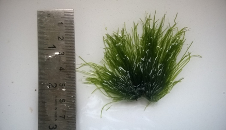
Grateloupia lithophila Borgesen, 1938 |
 |
 |
Kingdom |
Plantae |
Phylum |
Rhodophyta |
Class |
Florideophyceae |
Order |
Halymeniales |
Family |
Halymeniaceae |
Description: |
Blades are long and irregular tapering at the end, grows 10-15 cm long, slimy to touch, forms tuft on hard substratum. |
Worldwide distribution: |
Yemen, Sri Lanka, Indonesia |
Distribution along Indian coats: |
Goa, Maharashtra, Karnataka. |
Distribution along Uttara Kannada coast: |
Mugli-Honnavar; Kirubele, Belekan- Kumta; Honey beach-Ankola |
Habitat: |
Found in intertidal area, and tidal pools |
Growth seasons |
Occurs in mid Monsoon, easily dried up during prolonged emersion periods. |
Economical Uses: |
Potential feedstock for Bioethanol production |
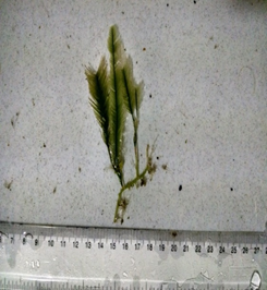
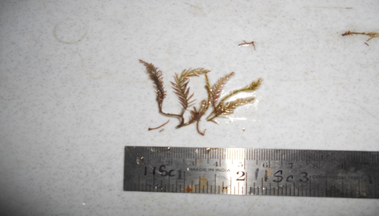
Gelidiopsis varaiabilis (Greville ex J. Agardh) F. Schmitz ,1895 |
|
Kingdom |
Plantae |
Phylum |
Rhodophyta |
class |
Florideophyceae |
Order |
Rhodymeniales |
Family |
Lomentariaceae |
Description: |
Thalli erect, about 4 cm high, composed of a few, irregularly branched cylindrical branches. |
Worldwide distribution: |
Diego Garcia atoll, Indonesia, Madagascar ,Seycelles, South Africa Sri Lanka |
Distribution along Indian coats: |
Lakshadweep, Kerala , Tamil Nadu ( Tuticorin , Kaniyakumari , Mandapam ) , Maharashtra ( Bombay ) , Andra Pradesh , Jalleshwar , Okha ( Gujarat ) Madagascar , |
Distribution along Uttara Kannada coast: |
Majali (Karwar), Mugli (Honnavar),Vannali (Kumta)
|
Growth seasons |
Post monsoon |
Habitat: |
Found in intertidal zone in Rocky shores |
Economical Uses: |
Agar production |
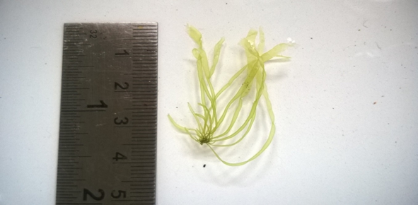
Gelidium pusillum (Stackhouse) Le Jolis, 1863 |
|
|
Kingdom |
Plantae |
Phylum |
Rhodopyta |
Class |
Florideophyceae |
Order |
Gelidiales |
Family |
Gelidium |
Description: |
Small plant grows upto 2-5 cm, forms tuft on substrata, blade is slightly long and flattened at the tip, sparsely pinnately proliferating. Blackish-red colour when dry, extensive rhizoids and flattened reproductive fronds |
Vernacular name: |
Small agar algae (Norwegian Bokmal) |
Worldwide distribution: |
France, Gulf of Mexico, Indian Ocean, Ireland, Kenya, Mediterranean Sea, North Atlantic Ocean, North Sea, Republic of Mauritius, Tanzania |
Distribution along Indian coast: |
Dwarka, Porbandar, Veraval (Gujarat), Mumbai (Maharashtra), Lakshadweep , Karnataka |
Distribution along Uttara Kannada coast: |
Majali- Karwar; Mugli – Honnavar |
Habitat: |
Found on exposed hard substratum in intertidal area. |
Growth season |
Occurs throughout all the seasons, peak growth in Pre monsoon |
Economic uses: |
Potential feedstock for bioethanol production also potential species as source of agar
|
|
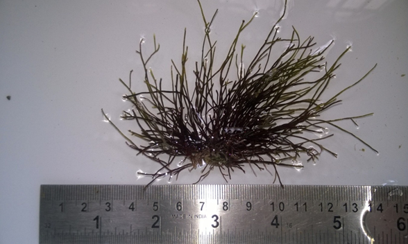
Hypnea valentiae (Turner) Montagne, 1841 |
 |
Kingdom |
Plantae |
Phylum |
Rhdophyta |
Class |
Florideophyceae |
Order |
Gigartinales |
Family |
Cystocloniaceae |
Description: |
Plant is erect and firmly branched. Branches are simple and thread like but occasionally forked and are distinctly oriented at right angle to the axis; inflated branches are seen as swollen bands at the middle, near the base or rarely near the tips of the ultimate branchlets |
Worldwide distribution: |
Aegean Sea, Gulf of Mexico, Indian Ocean, Kenya, Madagascar, Mediterranean Sea, North Atlantic Ocean, Republic of Mauritius, Seychelles, Tanzania |
Distribution along Indian coast: |
Bombay, Malvan, Ratnagiri, (Maharashtra) Goa, Karnataka, Lakshadweep. |
Distribution along Uttara Kannada coast: |
Majali- Karwar; Om beach – Kumta. |
Habitat: |
Mangrove swamps and Intertidal zone |
Growth season |
Monsoon and Post monsoon |
Economic Uses: |
It is a carrageenan yielding plant. This seaweed is also edible and the freshly gathered seaweed is commonly prepared as salad. Potential feedstock for biofuel production
|
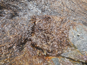
Chondria armata (Kutzing) Okamura, 1907
|
Kingdom |
Archaeplastida |
Phylum |
Rhodophyta |
Class |
Florideophyceae |
Order |
Ceramiales |
Family |
Rhodomelaceae |
Description: |
Thallus simple or branched, attached to rocky substratum by conical hold fast and clumps of rhizoids, branches with pinnately sub divided fronds which are arranged alternately in two opposite vertical rows. Tip of the branches bears hair-like structure when young, prominent but rarely persistent when old |
Worldwide distribution: |
Indian ocean, Kenya, Mozambique, South Africa, Tanzania |
Distribution along Indian Coast: |
Maharashtra (Bombay), Tamil Nadu (Tuticorin, Krusadai Island), Gujarat (Okha, Dwarka, Gulf of Kutch, Saurashtra), Goa, Lakshadweep Island, Andra Pradesh, Karnataka, Kerala. |
Distribution along Uttara Kannada Coast: |
Om beach-Kumta; Mugli- Honnavar |
Habitat: |
Intertidal zone in the lower parts of rocky shore |
Growth season: |
Throughout all the seasons |
Economical uses: |
Pharmaceuticals for glycoglycerolipid extraction |
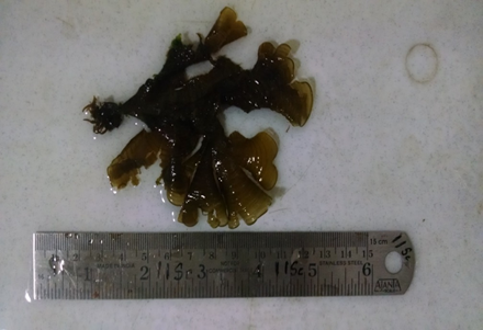
Gracilaria corticata (J. Agardh) J. Agardh, 1852 |
 |
 |
Kingdom |
Archaeplastida |
Phylum |
Rhodopyta |
Class |
Florideophyceae |
Order |
Gracilariales |
Family |
Gracilariaceae |
Description: |
Plants 10-12cm long, the thallus consists of bundles of flat and much divided blades with 2-3 mm broad segments; branching is dichotomous in young blades; in older plants numerous marginal projections line the edges of the segments in a pinnate fashion; they are ½-2 cm long; the colour of the plants vary from deep purple to grass green. |
Worldwide distribution: |
Indian ocean, Kenya, Madagascar, Republic of Mauritius, Tanzania. |
Distribution along Indian Coast: |
Dwarka, Okha (Gujarat), Bombay, Malvan, Ratnagiri, (Maharashtra) Goa, Karnataka. |
Distribution along Uttara Kannada Coast: |
Majali- Karwar; Dhareshwar, Mugli- Honnavar, Murudeshwar, Apsarkonda – Honnavar |
Habitat: |
Intertidal and subtidal zone |
Growth season |
Observed during all the seasons with peak growth in Post monsoon and Pre Monsoon. |
Economical Uses : |
It can be used for agar production, food, animal feed |
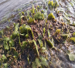
Padina tetrastromatica Hauck, 1887 |
 |
Kingdom |
Chromista |
Phylum |
Ochrophyta |
Class |
Phaeophyceae |
Order |
Dictyotales |
Family |
Dictyotaceae |
Description: |
Thalli divided into several small lobes, regularly and distinctly concentrically zonate; easily recognized due to dark double lines of sporangia; enclosing a line of colourless hairs in between; blades composed of two layers of cells. |
Worldwide distribution: |
Mediterranean Sea (Eastern basin), Federal Republic of Somalia, Kenya, Seychelles, South Africa, Tanzania. |
Distribution along Indian Coast: |
Gujrat, Malvan, Ratnagiri, (Maharashtra), Goa, Karnataka, Lakshadweep, |
Distribution along Uttara Kannada Coast: |
Karwar , Honnavar , Bhatkal |
Habitat: |
Mangrove swamps (attached to mud)/Intertidal and on sandy shores |
Growth seasons |
Growth period Mid Monsoon, peak growth in Post Monsoon |
Economical Uses: |
Extraction of alginate, fertilizer |
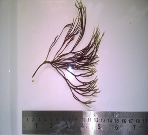
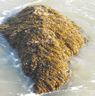
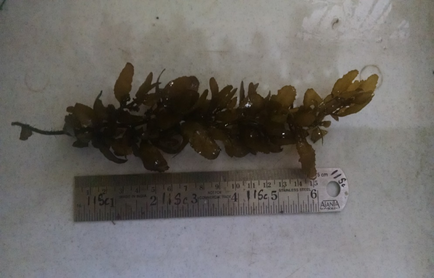
Sargassum ilicifolium (Turner) C.Agardh, 1820 |
|
|
Kingdom |
Chromista |
Phylum |
Ochrophyta |
Class |
Phaeophyceae |
Order |
Fucales |
Family |
Sargassaceae |
Description:
|
Plants 30-40 cm high with elliptical leaves in the upper part of the plant, 1-3 cm long and 8-15 mm broad; the margin is toothed, with minute and larger teeth mixed; midrib is visible for 2/3 of the length of the leaf, vanishing near the tip; branches are provided with spiny outgrowths; vesicles are nearly globular, 3-5mm in diameter with a stalk of the same length. |
Worldwide distribution: |
Kenya, Madagascar, Republic of Mauritius, Seychelles, South Africa, Tanzania. |
Distribution along Indian Coast: |
Gujarat, Malvan, (Maharashtra), Goa, Karnataka, Lakshadweep, |
Distribution along Uttara Kannada Coast: |
Majali- Karwar; Honnavar , Bhatkal . |
Habitat: |
Mangrove swamp, Intertidal in open coast. |
Growth season: |
Growth period Mid Monsoon, peak growth in Post Monsoon |
Economic uses: |
Used as a source of alginate, fertilizer, medicine and animal feed |
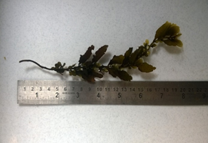
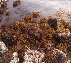
Sargassum cinereum J.Agardh, 1848 |
 |
Kingdom |
Chromista |
Phylum |
Ochrophyta |
Class |
Phaeophyceae |
Order |
Fucales |
Family |
Sargassaceae |
Description: |
Plants with short, stout main axis, bearing terate, smooth, primary branches at their upper part, beset with secondary branches and branchlets; basal leaves membranaceous, oblong, about 2.5 - 3 cm long, 7 - 8 mm broad, rounded at the apices and dentate at the margins; leaves of the branchlets lanceolate, 2 - 2.5 cm long, 3 - mm broad, cuneate at the base. Vesicles spherical, about 4 mm diameter, obovate, rounded, usually mucronate at the apices, sub cylindrical below. |
Worldwide distribution: |
Laccadive island, Sri Lanka, Indonesia, Mauritius |
Distribution along Indian Coast: |
Malvan, Ratnagiri, (Maharashtra). Goa, Karnataka, Kerala. |
Distribution along Uttara Kannada Coast: |
Vannalli rocky shore-Kumta , Honnavar , Bhatkal , Majali rocky shore-Karwar |
Habitat: |
Intertidal zone |
Growth season: |
Growth period Mid Monsoon, peak growth in Post Monsoon |
Economical Uses : |
Used as a source of alginate, fertilizer, medicine |
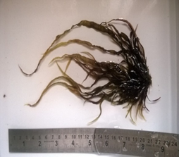
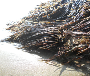
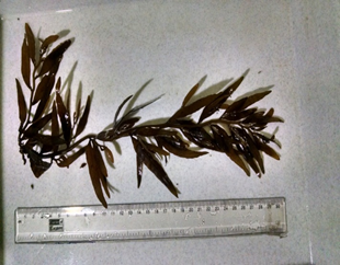
Sargassum wightii Greville ex J. Agardh, 1848 |
 |
|
Kingdom |
Chromista |
Phylum |
Ochrophyta |
Class |
Phaesophyceae |
Order |
Fucales |
Family |
Sargassaceae |
Description:
|
Plant dark-brown, 20-30 cm in height with a well-marked holdfast, upper portion richly branched, axes cylindrical, glabrous, leaves 5-8 cm long and 2-9mm broad, leaves tapering at the base and apex, midrib inconspicuous vesicles large, spherical or ellipsoidal being 5-8mm long and 3-4 mm broad, stipe of the vesicle 5-7 mm long seldom ending into a long tip, receptacles in clusters and repeatedly branched. |
Worldwide distribution: |
Indian Ocean. |
Distribution along Indian Coast: |
Bombay(Maharashtra) , Goa, Karnataka , Kerala. |
Distribution along Uttara Kannada Coast: |
Majali- Karwar |
Habitat: |
Intertidal and subtidal |
Growth season: |
Growth period Mid Monsoon, peak growth in Post Monsoon |
Economical Uses: |
It is used as raw material for the production of sodium alginate. It also contains 8-10 % of mannitol which can be used as substitute for sugar, fertilizer and medicine
|
Dictyota bartayresiana J.V. Lamouroux, 1809 |
 |
Kingdom |
Chromista |
Phylum |
Ochrophyta |
Class |
Phaeophyceae |
Order |
Dictyotales |
Family |
Dictyotacea |
Description: |
Plants 9-14 cm high, erect, not entangled, a little harsh to the touch, attached to the substratum by irregularly shaped holdfast with rhizoids, thallus branched dichotomously; segments without midrib, 1 to 1.5 cm long, 2 - 4 mm broad above a fork, broadening to 6 - 10 mm below the next fork; margin entire, tips are pointed except in young branches. Sporangia 125 - 140 µ in diameter. |
Worldwide distribution: |
Gulf of Mexico , Indian ocean , Kenya ,Madagascar, Mozambique , New Zealand , North Atlantic ocean , Republic of Mauritius , Seychelles , Tanzania . |
Distribution along Indian Coast: |
Okha (Gujrat), Malvan, Ratnagiri, (Maharashtra), Goa, Karnataka, Lakshadweep |
Distribution along Uttara Kannada Coast: |
Karwar , Honnavar , Bhatkal |
Habitat: |
Intertidal zone |
Growth season: |
Growth period Mid Monsoon, peak growth in Post Monsoon |
Economical Uses: |
Food, animal feed and alginate production |
3. Seaweed genera identification Key
Key to common Genera of Chlorophyta
1. Plant hollow and tubular, one celled thick......................................Enteromorpha.
Plant membranous ....................................................................2.
2. Plant membranous, 2 celled thick ..................................................Ulva.
Plant filamentous, unbranched thick cell wall .........................3.
3. Plant filamentous, thick cell wall, basal cell long
compared with the width, unbranched................................................Chaetomorpha.
Plant filamentous branched ......................................................4.
4. Plant filamentous tufted branched,
lower branches dichotomous ..............................................................Cladophora
Plant coenocytious. ..................................................................5.
5. Plant coenocytious organized to form
stolon and erect branches ....................................................................Caulerpa
Key to common Genera of Phaeophyta
6. Plant erect, dichotomously branched with rounded
apex, unilocular sporangia ....................................................................Dictyota
Plant broad, sparsely branched without mid-rib..........................7.
7. Plant broad, erect, margin entire, branches
irregularly dichotomus ..........................................................................Spatoglossum
Plant entire, lobbed .....................................................................8.
8.Plant entire, lobbed,2-8 celled thick marked with
concentric row of hairs .......................................................................... Padina
Plant erect, axis cylindrical bearing leaves and vesicles .............9
9. Plant with erect axis, branched, leaves membranous,
prominent mid rib, receptacles axially ................................................... Sargassum.
Key to common Genera of Rhodophyta
10. Plant erect, foliaceous, margin entire, majenta colour,
stallate chloroplast with central pyrenoid .....................................................Porphyra
Plant tufted, dichotomously branched ............................................11.
11. Plant cartilaginous, terate to compress, saxicolous .................................Gelidium
Plant slender, cylindrical stolon .....................................................12.
12. Plant cartilaginous, erect, stolon give rise to erect and
decumbent branches above and coarse short rhizoidal
branches below, axial branches are cylindrical or compressed,
stichidia are borne on the swollen tips ............................................................Gelidiella
Plant bushy, wiry clumps .................................................................13.
13. Plant bushy, wiry clumps, lower branches some what
creeping, upper erect tapering towards the apex ..............................................Gelidiopsis
Plant branched, axis cylindrical or flattened.....................................14.
14. Plant branched, flattened, structurally composed of
central medulla surrounded by cortex ...............................................................Gracilaria
Plant cylindrical, profusely branched bearing
short acute alternate branches ...........................................................15.
15. Plant erect radially branched, cylindrical, commonly
beset with numerous thorn like branchelets. Tetraspores
and cystocarps in swollen alternate branches......................................................Hypnea
Plant erect, cartilaginous, wart like determinate branchlets...............16
16.Plant erect, cartilaginous, determinate branches
beset with wart like branchlets ............................................................................Laurentia
Plant erect, cylindrical, determinate branches acute..........................17
17. Plant erect, cylindrical, delicate in texture, determinate
branches acute, stalked antheridia, oval cystocrap ..............................................Chondria
Plant erect, flattened to foiliaceous ...................................................18.
18. Plant erect, flattened with slippery blade, branches
pinnate to irregular, texture firm, dark purple colour ............................................Grateloupia
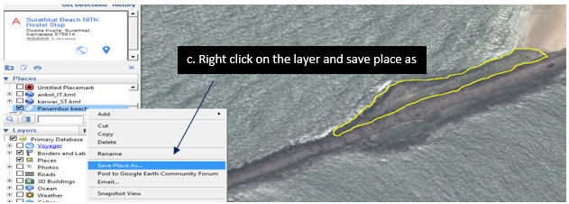
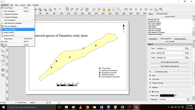
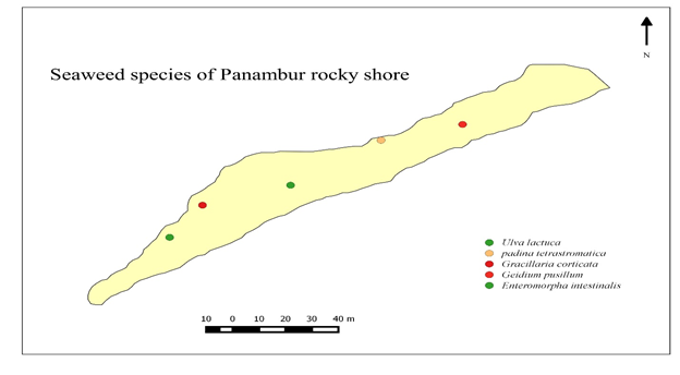
9.1. SPATIAL MAPPING -SEAWEEDS DISTRIBUTION
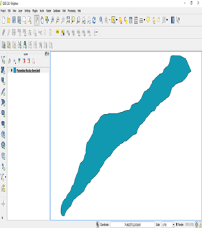
9.1.1. Digitizing the Rocky shores
1. Downloading google earth (http://www.google.com/earth/)
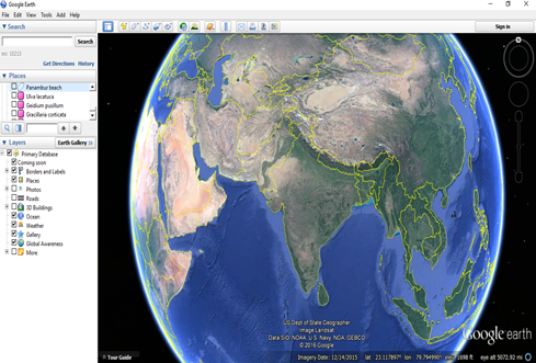
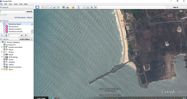
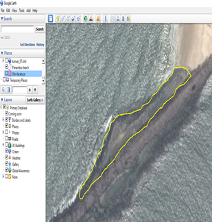
9.1.2. Installing Google earth


Zoom to the desired location /rocky shore
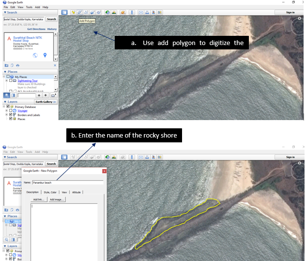
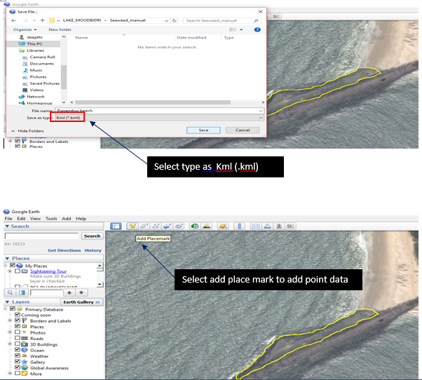
9.1.3. Using the polygon tool digitized the rocky shore
QUANTUM GIS (QGIS) – SPATIAL MAPPING TOOL
QGIS is a Free and Open Source GIS for manipulating geographical data (vector, raster), statistical analysis.
Downloading and Installing QGIS
- Download QGIS from http://www.qgis.org/en/site/
- Click on download now you will find the list of versions available.
- Download the latest stable version.

- QGIS main page will be opened as shown below.
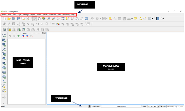
- The menu bar provides access to numerous QGIS features.
- The toolbars offer additional tools for interacting with the map. Hold the mouse over the particular icon, a short description of the tool’s purpose will be displayed.
- The map legend area sets the visibility
- The map overview panel provides a full extent view of layers added
- The status bar shows the current position in map coordinates
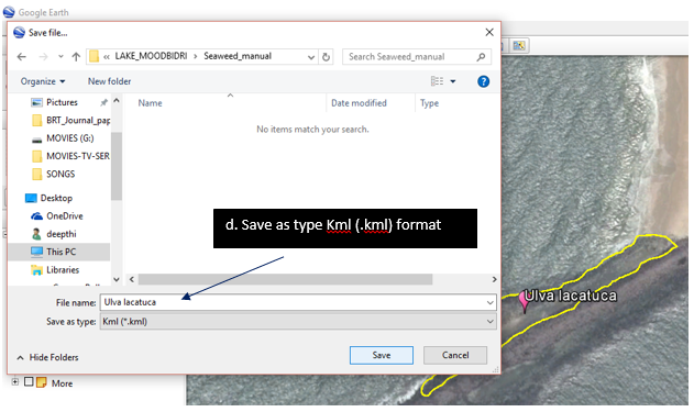
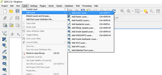
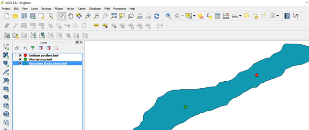
Importing vector layer (.kml file)
- Click on add layer go to add vector layer

Import the .kml file by browsing
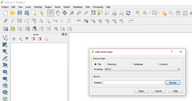
If the file is not visible click on keyhole markup language [KML] (*.kml *KML)

Vector layer displayed in the map overview
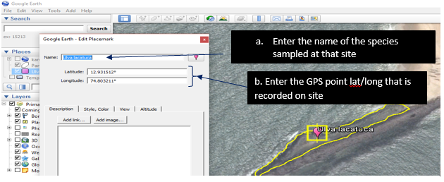
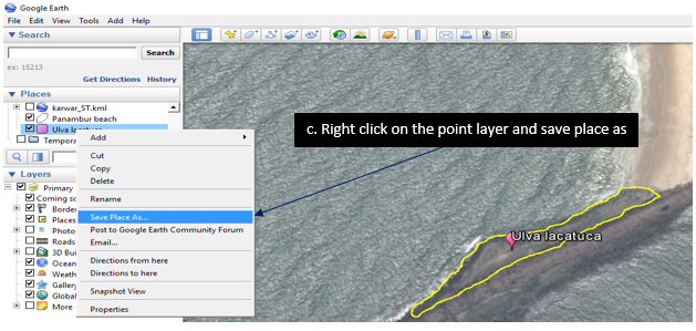
In a similar way import the point data in this case the seaweed species data
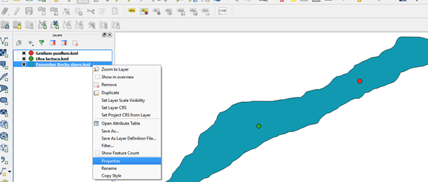
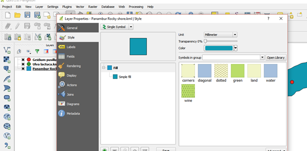
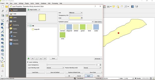
Layer properties such as size, colour, label, font can be edited
- right click on the layer go to properties
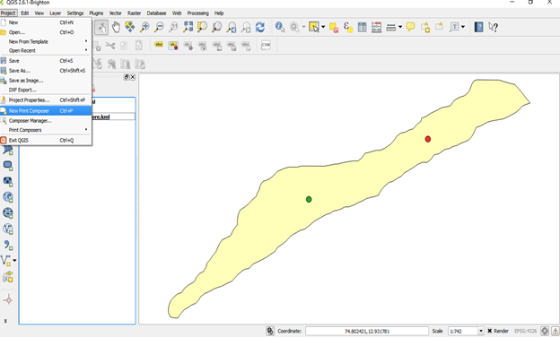
For final map representation
- Go to project click on new map composer
- Give id as 1 a new map window opens
Add new map by dragging the cursor inside the window
- On the left hand side different icons are present which helps in adding legend, label and direction
- On right hand side these icons are edited in item properties
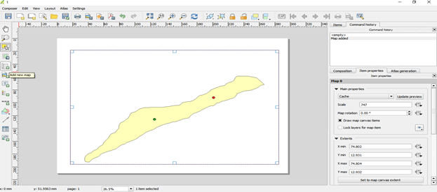
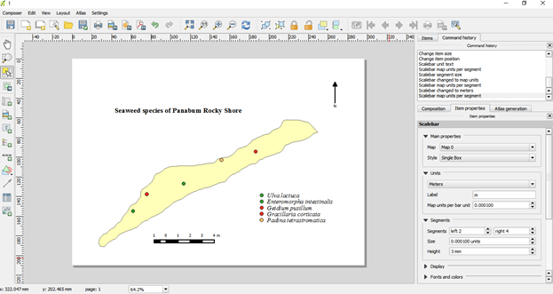
Final map can be saved as jpg image
Help from QGIS:
http://www.qgis.org/en/site/forusers/index.html#
http://www.qgis.org/en/docs/index.html
References:
NIO bioinformatics-http://www.niobioi
« »
PROTOCOL FOR WATER QUALITY MONITORING (PHYSICAL, CHEMICAL AND BIOLOGICAL PARAMETERS)
WATER SAMPLING
|
Sampling:
The sample collected should be small in volume, enough to accurately represent the whole water body. The water sample tends to modify itself to the new environment. It is necessary to ensure that no significant changes occur in the sample and preserve its integrity till analysed (by retaining the same concentration of all the components as in the water body). The essential objectives of water quality assessment are to:
- Define the status and trends in water quality of a given water body.
- Analyse the causes for the observed conditions and trends.
- Identify the area specific problems of water quality and provide assessments in the form of management to evaluate alternatives that help in decision-making.
|
Site selection in a waterbody: Sampling sites for the water body/lake are selected to represent the water quality at different points and depths. Generally three sampling sites are selected for monitoring.
- Inlet: the point where the principal feeder opens into the lake.
- Center: the point that gives the general water quality of the lake.
- Outlet: the place where the overflow occurs.
|
Types of sampling: Generally three types of sampling are adopted for collecting water samples.
- Grab or Catch sampling: the sample is collected at a particular time and place that represents the composition of the source at that particular point and time.
- Composite sampling: a mixture of grab samples is collected at the same sampling point at different time intervals.
- Integrated sampling:a mixture of grab samples collected at different points simultaneously.
|
Sampling frequency
The quality of water varies with time in a water body due to various natural and human induced factors. The monitoring has to be done in a way that records all the changes in the quality. The sampling frequencies generally adopted in monitoring are:
- Monthly sampling covering all seasons (preferably for 24 months).
- Weekly sampling for one year.
- Consecutive day sampling during the study period.
- Hourly sampling for 24 hours (example: parameters such as dissolved oxygen, pH, etc.).
|
Variations in water quality are mainly due to changes in the concentrations of the components of the water flowing into the water body. These variations can be man-made or natural and can either be cyclic or random.
- Random variations: due to spasmodic, often unpredictable events such as accidental oil spills, sewage leaks, overflows, etc.
- Cyclic variations: may be a result of regular seasonal changes triggering certain natural processes such as rainfall, snowmelts and seasonal temperature changes, altering the ecosystem. Seasonal growth and decay of vegetation will also rise due to cyclic changes in the composition of water.
In lakes, the mass of water and good lateral mixing provide inertia against any rapid modifications due to inputs and outputs. |
Sampling container: The sampling container should not react with the sample, be of adequate capacity to store the sample and be free from contamination. |
Sampling method: Grab sampling can be performed at the inlet, center and outlet in most of the water bodies studied to assess their physical and chemical qualities. The samples can be collected in thoroughly cleaned 2.5-litre inert plastic containers, which is rinsed with distilled and lake/tank water before collection.
Note: Water samples were collected in a sampling bottle avoiding floating materials. The stoppers of the sample containers were closed properly to prevent outside contamination. The container was labelled describing the name of the water body, date, time, sampling-point, and conditions under which it was sampled. |
Analyses of Physical, Chemical and Biological Parameters |
The parameters analysed to assess the water quality are broadly divided into:
- Physical parameters: Colour, Temperature, Transparency, Turbidity and Odour.
- Chemical parameters: pH, Electrical Conductivity (E.C), Total Solids (TS), Total Dissolved Solids (TDS), Total Suspended Solids (TSS), Total Hardness, Calcium Hardness, Magnesium Hardness, Nitrates, Phosphates, Chlorides, Dissolved Oxygen (D.O), Biological Oxygen Demand (BOD), Chemical Oxygen Demand (COD), Fluorides, Free Carbon-dioxide, Potassium and Sodium.
- Biological parameters: The biological parameters involved the qualitative analyses of planktons
|
Field measurement: The field (on-spot) parameters measured include pH, conductivity, dissolved oxygen, temperature and transparency. |
Sample Preservation: Between the time a sample is collected and analysed in the laboratory, physical, chemical and biochemical reactions may take place in the sample container leading to changes in the intrinsic quality of the sample, making it necessary to prevent or minimize these changes with suitable preservatives such as alcohol and mercuric chloride. Highly unstable parameters such as pH, temperature, transparency, free carbon-dioxide, dissolved oxygen, etc. is measured at the sampling site. The preservation procedure includes keeping the samples in the dark, adding chemical preservative, lowering the temperature to retard reactions, or combinations of these. |
Experiment |
Preservative |
Max. holding time |
BOD |
Cool, 4o C |
4 hours |
Calcium |
Cool, 4o C |
7 days |
Chloride |
Cool, 4o C |
7 days |
COD |
Cool, 4o C |
24 hours |
Dissolved Oxygen* |
Fix on site |
6 hours |
Magnesium |
Cool, 4o C |
7 days |
Nitrate + Nitrite |
Cool, 4o C |
24 hours |
pH |
None |
6 hours |
Phosphorus* |
|
|
Dissolved |
Filter on site using 0.45µm filter |
24 hours |
Inorganic |
Cool, 4o C |
24 hours |
Ortho |
Cool, 4o C |
24 hours |
Total |
Cool, 4o C |
1 month |
Potassium |
Cool, 4o C |
7 days |
Specific Conductance |
Cool, 4o C |
24 hours |
Sodium |
Cool, 4o C |
7 days |
(Source: Analytical Methods Manual, Water quality branch, Environment Canada, 1981) |
WATER TEMPERATURE |
1 |
WATER TEMPERATURE: The water temperature is important for its effects on the chemistry, and biological reactions in the organisms in water. A rise in temperature of the water leads to the speeding up of the chemical reactions in water, reduces the solubility of gases, affects carbon dioxide-carbonate-bicarbonate equilibrium and amplifies the tastes and odours. Temperature influences water chemistry, e.g. DO, solubility, density, pH, alkalinity, salinity, conductivity etc. At elevated temperatures, metabolic activity of organism’s increases, requiring more oxygen but at the same time the solubility of oxygen decreases. Water temperature is important in relation to fish life. The disease resistance in the fishes also decreases with rise in temperature. The aquatic organisms show varied sensitivities to temperature. The temperature of drinking water has an influence on its taste. |
Procedure
Clean the pH-TDS-EC probe/thermometer (Hg bulb region) with distilled water and fill the container with water sample. Then check the water temperature of the sample by dipping the pH-TDS-EC probe into sample and record it in degrees Celsius (ºC). |
Apparatus: pH-TDS-EC probe/ Laboratory thermometer, Beaker |
Do’s and Dont’s:
- Clean the electrode (sensor parts) of the meter with distilled water and wipe properly using tissue paper, before and after usage.
- Calibrate the meters prior to each field trip. (Follow internal calibration solutions as per the Company instructions)
- Ensure: Company instructions for field use, maintenance and storage of the pH-TDS-EC probe have been followed properly.
- Note down the temperature readings of each sample.
- Don’t expose the meter/laboratory thermometer directly to sunlight.
|
Results |
Date |
S1 |
S2 |
S3 |
|
Limits (Inland) |
|
|
|
|
|
|
Inference |
|
References |
APHA (1998); Trivedi R. K. and Goel P. K. (1986); Ramachandra T. V. and Ahalya N. (2001) |
pH: pH is the measure of the acid-base balance of a solution and is defined as the negative logarithm to the base 10 of the hydrogen ion (H+) concentration. The pH scale runs from 0 to 14 (i.e., very acidic to very alkaline) with pH 7 representing a neutral solution. When the pH is less than 7, it is said to be acidic; a pH greater than 7 is basic.
pH tends to increase during day largely due to the photosynthetic activity (consumption of carbondioxide) and decreases during night due to respiratory activity. pH is also governed by the equilibrium between carbon dioxide/bicarbonate/carbonate ions. The change in the intensity of acidity or alkalinity of an aquatic ecosystem can be due to inflow of industrial effluents, domestic sewage and atmospheric deposition of acid-forming substances. Diurnal variations in pH can take place due to photosynthesis and respiration cycles of algae in eutrophic waters. Acidity of water is controlled by strong mineral acids, weak acids (such as carbonic, humic and fulvic acids) and hydrolysing salts of metals such as iron and aluminium. Waste water and polluted natural waters have pH values lower or higher than 7 based on the nature of the pollutant. Changes in pH endanger the lives of the organisms in the water.
A lower pH value, below 4 will produce sour taste whereas pH above 8.5 produces an alkaline taste. If the pH is below 6.5, corrosion of pipes occur, thus toxic metals like Zinc, Lead, Cadmium and Copper etc. are released. Higher pH values induce scale formation in water heating apparatus, production of toxic trihalomethanes and also reduce the germicidal potential of chlorine. |
Procedure
- Colorimetric method: About 10ml of the sample is taken in a wide mouth test tube, 0.2 ml of BDH indicator is added, and shaken gently. The colour developed is matched with the chart and the pH noted.
- Electrometric method: The pH is determined by measuring the Electro Motive Force (E.M.F) of a cell comprising an indicator electrode (an electrode responsive to hydrogen ions such as a glass electrode) immersed in the test solution and the reference electrode (usually a mercury/calomel electrode). Contact between the test solution and the reference electrode is usually got by means of a liquid junction, which forms a part of reference electrode. E.M.F of this cell is measured with pH meter that is a high impedance voltmeter calibrated in terms of pH. The electrode is allowed to stand for 2 minutes to stabilize before taking reading for reproducible results (at least ±0.1 pH units).
|
Apparatus:
- pH indicator (BDH) method: BDH Indicator (Universal Indicator) and test tubes.
- Electrometric method: Glass electrode, reference electrode (mercury/calomel or silver/silver chloride) and pH meter.
|
Do’s and Dont’s:
- Clean the meters with distilled water and wipe properly using tissue paper, before and after usage.
- Calibrate the meters prior to each field trip.
- Ensure that all the instructions on use, maintenance and storage of the pH-TDS-EC probe have been followed.
- Note down the pH readings of each sample.
|
Results |
Date |
S1 |
S2 |
S3 |
|
Limits (Inland) |
|
|
|
|
|
Permissible
7-8.5
Excessive
Not less than 6.5 or greater than 9.2 |
Inference |
|
References |
APHA (1998); Trivedi R. K. and Goel P. K. (1986); Ramachandra T. V. and Ahalya N. (2001) |
ELECTRICAL CONDUCTIVITY (EC)
|
3 |
ELECTRICAL CONDUCTIVITY: Conductivity denotes the ability of an aqueous solution to conduct an electrical current. It depends on the presence of ions, their total concentration, mobility, valence, relative concentration and on the temperature of measurement. Electrolytes in a solution dissociate into positive (cations) and negative (anions) ions and impart conductivity. Solution of most inorganic acids, bases and salts (chloride, nitrate, sulfate, phosphate anions, sodium, magnesium, calcium, iron, and aluminium cations) are relatively good conductors unlike organic compounds (oil, phenol, alcohol, and sugar). Conductivity increases with temperature.
Conductance is defined as the reciprocal of the resistance involved and expressed as mho or Siemen (s).
G=1/R [where, G – Conductance (mho or Siemens) and R – Resistance]
The amount of current that can flow through a solution is proportional to the concentration of dissolved ionic species in the solution. Thus, higher the concentration of electrolytes in water, the more is its electrical conductivity. i.e. lesser the resistance. |
Procedure
The electrode of the conductivity meter is dipped into the sample, and the readings are noted for stable value shown as mS/cm. |
Apparatus: Conductivity meter, 100ml Beaker |
Do’s and Dont’s:
- Clean the meters with distilled water and wipe properly using tissue paper, before and after usage.
- Calibrate the meters prior to each field trip.
- Ensure that all the instructions on use, maintenance and storage of the pH-TDS-EC probe has been followed.
- Note down the EC readings of each sample.
|
Results |
Date |
S1 |
S2 |
S3 |
|
Limits (Inland) |
|
|
|
|
|
Permissible
750-2000
Excessive
>2000 |
Inference |
|
References |
APHA (1998); Trivedi R. K. and Goel P. K. (1986); Ramachandra T. V. and Ahalya N. (2001) |
TOTAL DISSOLVED SOLIDS (TDS) |
4 |
TDS : The substances that would pass through the filter paper but will remain as residue when the water evaporates which includes dissolved minerals and salts, humic, tannin and pyrogens. A constant level of minerals in the water is necessary for aquatic life. Changes in the amounts of dissolved solids can be harmful because the density of total dissolved solids determines the flow of water in and out of an organism’s cells. Many of these dissolved solids contain chemicals, such as nitrogen, phosphorous, and sulfur, which are the building blocks of molecules for life. Concentration of total dissolved solids that are too high or too low may limit the growth and may lead to the death of many aquatic organisms. High concentrations of total dissolved solids may reduce water clarity, which contributes to a decrease in photosynthesis and lead to an increase in water temperature. Many aquatic organisms cannot survive in high temperatures. The conductivity in water is affected by the presence of inorganic dissolved solids such as chloride, nitrate, sulfate, and phosphate anions or sodium, magnesium, calcium, iron, and aluminum cations. These particles contribute the dissolved solids of the water. Waters with high dissolved solids generally are of inferior palatability and may induce an unfavourable physiological reaction. |
Procedure
Clean the pH-TDS-EC probe with distilled water and fill the container with water sample. Then the total dissolved solids is determined by dipping the pH-TDS-EC probe into sample and express in parts per million (ppm). |
Apparatus: pH-TDS-EC probe, 100ml Beaker |
Do’s and Dont’s:
- Clean the meters with distilled water and wipe properly using tissue paper, before and after usage.
- Calibrate the meters prior to each field trip.
- Ensure that all the instructions on use, maintenance and storage of the pH-TDS-EC probe has been followed.
- Note down the TDS readings of each sample.
|
Results |
Date |
S1 |
S2 |
S3 |
|
Limits (Inland) |
|
|
|
|
|
Permissible
500
Excessive
1500 |
Inference |
|
References |
APHA (1998); Trivedi R. K. and Goel P. K. (1986); Ramachandra T. V. and Ahalya N. (2001) |
TRANSPARENCY (LIGHT PENETRATION) |
5 |
TRANSPARENCY: Solar radiation is the major source of light energy in an aquatic system, governing the primary productivity. Transparency is a characteristic of water that varies with the combined effect of colour and turbidity. It measures the light penetrating through the water body and is determined using Secchi disc. |
Procedure
Transparency is measured by gradually lowering the Secchi disc at respective sampling points. The depth at which it disappears in the water (X1) and reappears (X2) is noted.
The transparency of the water body is computed as follows:
Transparency (Secchi Disc Transparency) = (X1 + X2 )/2
Where, X1 = Depth at which Secchi disc disappears
X2 = Depth at which Secchi disc reappears |
Apparatus: Secchi disc, a metallic disc of 20cm diameter with four quadrats of alternate black and white on the upper surface. The disc with centrally placed weight at the lower surface, is suspended with a graduated cord at the center.
|
Do’s and Dont’s:
- Clean the secchi disc before and after usage.
- Handle the secchi disc with care.
- Note down the readings of each sample.
|
Results |
Date |
S1 |
S2 |
S3 |
|
Limits (Inland) |
|
|
|
|
|
Permissible
Excessive |
Inference |
|
References |
APHA (1998); Trivedi R. K. and Goel P. K. (1986); Ramachandra T. V. and Ahalya N. (2001) |
TURBIDITY |
6 |
TURBIDITY: Turbidity is an expression of optical property; wherein light is scattered by suspended particles present in water (Tyndall effect) and is measured using a nephelometer. Any substance having a particle size more than 10‑9 will produce turbidity in water. Suspended and colloidal matter such as clay, silt, finely divided organic and inorganic matter; plankton and other microscopic organisms cause turbidity in water. Turbidity affects light scattering, absorption properties and appearance in a water body. Increase in the intensity of scattered light results in higher values of turbidity. Turbidity makes the water unfit for domestic purposes, food and beverage industries, and many other industrial purposes. In natural waters, turbidity restricts light penetration for photosynthesis.
Nephelometric measurement is based on comparison of the intensity of scattered light of the sample with the intensity of light scattered by a standard reference suspension (Formazin polymer) under similar conditions. |
Procedure: The nephelometer is calibrated using distilled water (Zero NTU) and a standard turbidity suspension of 40 NTU. The thoroughly shaken sample is taken in the nephelometric tube and the value is recorded.
Turbidity (NTU) = (Nephelometer readings) (Dilution factor*)
* If the turbidity of the sample is more than 40 NTU, then the sample is diluted and the dilution factor is accounted in final calculations. |
Apparatus:Nephelometer (It detects scattered light at 90o to the incident beam of light. It consists of a light source for illuminating the sample. One or more photoelectric detectors with a display unit indicate the intensity of light scattered at 90o to the path of incident light.), sample cells, lab-glass wares. |
Do’s and Dont’s:
- Collect the sample directly into the sampling cuvet (cell).
- Do not leave the sample cell in the meter so as to avoid scratches.
- Empty the sample at each site and rinse properly.
- Note down the Turbidity readings of each sample.
- Wipe the cell properly with tissue paper and ensure that the outside of the cell is clean and dry before placing the cell in to the meter.
|
Results |
Date |
S1 |
S2 |
S3 |
|
Limits (Inland) |
|
|
|
|
|
Permissible
5 NTU
Excessive
25 NTU |
Inference |
|
References |
APHA (1998); Trivedi R. K. and Goel P. K. (1986); Ramachandra T. V. and Ahalya N. (2001) |
DISSOLVED OXYGEN (DO) |
7 |
DISSOLVED OXYGEN: Oxygen is essential to all forms of aquatic life. DO depend upon the physical, chemical and biochemical activities in the water body. The analysis of DO is a key test in water pollution and waste treatment control. The two main sources of dissolved oxygen are diffusion of oxygen from the air and photosynthetic activity. Low levels of DO frequently indicate a high concentration of decaying organic matter in the water. As bacteria digest organic matter, they use up oxygen, leaving little for the other aquatic creatures. The factors affecting the DO are (1) temperature: as temperature increases, the amount of oxygen (or any gas) dissolved in water decreases. (2) Partial pressure of O2 in contact with water: at high altitudes, less oxygen is dissolved in water because the partial pressure of oxygen in the atmospheric is low (3) Salinity: the solubility of gases O2 and CO2 decreases with increasing salinity.
D.O (mg/L) |
Water quality |
Above 8.0 |
Good |
6.5-8.0 |
Slightly polluted |
4.5-6.5 |
Moderately polluted |
4.0-4.5 |
Heavily polluted |
Below 4.0 |
Severely polluted |
Winkler’s method
Principle: Oxygen present in the sample oxidizes the dispersed divalent manganous hydroxide to the higher valency to precipitate as a brown hydrated oxide after addition of potassium iodide and sodium hydroxide. Upon acidification, manganese reverts to its divalent state and liberates iodine from potassium iodide, equivalent to the original dissolved oxygen content of the sample. The liberated iodine is titrated against N/80 sodium thiosulphate using fresh iodine as an indicator. |
Calculation: NIVI = N2V2 (Molar equivalence formula)
(ml*N) of sodium thiosulphate * 8 * 1000
 Dissolved oxygen, mg/L = Dissolved oxygen, mg/L =
V2 [(V1 - V)/V1]
Where, V1 = Volume of sample bottle
V2 = Volume of contents titrated
V = Volume of MnSO4 and KI added (2ml)
Procedure
The samples are collected in BOD bottles, to which 1ml of manganous sulphate and 1ml of potassium iodide are added and sealed. This is mixed well and the precipitate is allowed to settle down. Then, 1ml of concentrated sulphuric acid is added, and mixed well until all the precipitate dissolves. 25 ml of the sample is measured into the conical flask and titrated against 0.025N sodium thiosulphate using starch as an indicator. The end point is the change of colour from blue to colourless. |
Apparatus: BOD bottle-125ml, measuring cylinder, conical flask, 1ml glass pipette etc. |
Reagents:
Manganous sulphate solution: Dissolved 100 g of manganous sulphate in 200ml of distilled water and heated to dissolve salt and filtered after cooling.
- Alkaline potassium iodide solution: Dissolved 100 g of KOH and 50 g of KI in 200ml of pre-boiled distilled water.
- Starch indicator:1g of starch is dissolved in 100 ml of warm distilled water and added few drops of formaldehyde solution.
- Stock sodium thiosulphate (0.1 N):24.82g of sodium thiosulphate pentahydrate (Na2S202. 5H2O) is dissolved in distilled water and made up to 1000ml.
- Standard sodium thiosulphate (0.025N): 250ml of the stock sodium thiosulphate pentahydrate is made up to 1000ml with distilled water to give 0.025N.
|
Do’s and Dont’s
- Label the BOD bottle with waterproof pen before collecting sample.
- Ensure that no air bubble enters the BOD bottle while filling it with water sample.
- Clean and different microtips should be used for each reagent.
- Handle the reagents and acids with extreme care. Wear disposable gloves if possible.
- Don’t keep the BOD under direct sunlight while doing experiment as it will interfere with the results.
|
Results |
Date |
S1 |
S2 |
S3 |
|
Limits (Inland) |
|
|
|
|
|
Permissible
3
Excessive
6 |
Inference |
|
References |
APHA (1998); Trivedi R. K. and Goel P. K. (1986); Ramachandra T. V. and Ahalya N. (2001) |
BIOLOGICAL OXYGEN DEMAND (BOD) |
8 |
BIOLOGICAL OXYGEN DEMAND: BOD is the amount of oxygen required by microorganisms for stabilizing biologically decomposable organic matter (carbonaceous) in water under aerobic conditions. The test is used to determine the pollution load of wastewater, the degree of pollution and the efficiency of wastewater treatment methods. 5-Day BOD test being a bioassay procedure (involving measurement of oxygen consumed by bacteria for degrading the organic matter under aerobic conditions) requires the addition of nutrients and maintaining the standard conditions of pH and temperature and absence of microbial growth inhibiting substances.
The method consists of filling the samples in airtight bottles of specified size and incubating them at specified temperature (20 oC) for 5 days. The difference in the dissolved oxygen measured initially and after incubation gives the BOD of the sample.
Calculation:
BOD, mg/L = (D0 – D5) x Dilution factor
Where,
D0 = Initial DO in the sample
D5 = DO of the sample after 5 days |
|
Procedure
The sample having a pH of 7 is determined for first day DO. Various dilutions (at least 3) are prepared to obtain about 50% depletion of D.O. using sample and dilution water. The samples are incubated at 20 oC for 5 days and the 5th day D.O is noted using the Winkler’s method. A reagent blank is also prepared in a similar manner. |
Apparatus: BOD bottles - 125ml capacity, air incubator - to be controlled at 20 oC ± 1 oC, magnetic stirrer. |
Reagents:
- Manganous sulphate solution: Dissolved 100 g of manganous sulphate in 200ml of distilled water and heated to dissolve salt and filtered after cooling.
- Alkaline potassium iodide solution: Dissolved 100 g of KOH and 50 g of KI in 200ml of pre-boiled distilled water.
- Starch indicator:1g of starch is dissolved in 100 ml of warm distilled water.
- Stock sodium thiosulphate (0.1 N):24.82g of sodium thiosulphate pentahydrate (Na2S2O2. 5H2O) is dissolved in distilled water and made up to 1000ml.
- Standard sodium thiosulphate (0.025N): 250ml of the stock sodium thiosulphate pentahydrate is made up to 1000ml with distilled water to give 0.025N.
- Formaldehyde: preservative for freshly prepared starch solution
|
Do’s and Dont’s
- Rinse the BOD bottles properly with distilled water before initiating the experiment.
- Label the BOD bottle with waterproof labels/pen before collecting sample.
- Ensure that no air bubble enters the BOD bottle while filling it with water sample.
- Handle the reagents and acids with extreme care. Wear disposable gloves if possible.
- Don’t keep the BOD bottles under direct sunlight while doing experiment as it will interfere with the results.
*Alkaline KI – potential skin irritant
*Conc. H2SO4 – corrosive acid |
Results |
Date |
S1 |
S2 |
S3 |
|
Limits (Inland) |
|
|
|
|
|
Permissible 10
Excessive 30 |
Inference |
|
References |
APHA (1998); Trivedi R. K. and Goel P. K. (1986); Ramachandra T. V. and Ahalya N. (2001) |
CHEMICAL OXYGEN DEMAND (COD) |
9 |
CHEMICAL OXYGEN DEMAND: COD is the measure of oxygen equivalent to the organic content of the sample that is susceptible to oxidation by a strong chemical oxidant. The intrinsic limitation of the test lies in its ability to differentiate between the biologically oxidisable and inert material. It is measured by the open reflux method.
The organic matter in the sample gets oxidized completely by strong oxidizing agents such as potassium dichromate in the presence of conc. sulphuric acid to produce carbon-dioxide and water. The excess potassium dichromate remaining after the reaction is titrated with Ferrous Ammonium Sulphate (FAS) using ferroin indicator to determine the COD. The dichromate consumed gives the oxygen required for the oxidation of the organic matter. |
Procedure
15ml of conc. sulphuric acid with 0.3g of mercuric sulphate and a pinch of silver sulphate along with 5ml of 0.025M potassium dichromate is taken into a Nessler's tube. 10ml of sample (thoroughly shaken) is pipetted out into this mixture and kept for about 90 minutes on the hot plate for digestion. 40ml of distilled water is added to the cooled mixture (to make up to 50ml) and titrated against 0.25M FAS using ferroin indicator, till the colour turns from blue green to wine red indicating the end point. A reagent blank is also carried out using 10ml of distilled water.
Calculation:
 COD, mg/L = (b-a) x N of FAS x 1000 x 8 COD, mg/L = (b-a) x N of FAS x 1000 x 8
ml of sample
Where,
a = ml of titrant with sample.
b = ml of titrant with blank. |
Apparatus: Reflux apparatus, Nessler’s tube, Erlenmeyer flasks, hot plate and lab glassware. |
Reagents:
- Standard potassium dichromate solution (0.250M): 12.25g of potassium dichromate dried at 103 oC for about 2 hours is dissolved in distilled water and made up to 1000ml.
- Standard ferrous ammonium sulphate (FAS) 0.25N:98g of FAS is dissolved in minimum distilled water to which 20ml of conc. sulphuric acid is added and made up to 1000ml using distilled water to give 0.25N of ferrous ammonium sulphate.
- Ferroin indicator:1.485g of 1,10-Phenanthroline monohydrate and 695mg of ferrous sulphate is dissolved in 100ml of distilled water.
- Conc. sulphuric acid
- Silver sulphate crystal
- Mercuric sulphate crystals
|
Do’s and Dont’s
- Label the cleaned Erlenmeyer flasks properly.
.
- Handle the reagents and acids with extreme care.
- It is safe to wear gloves.
|
Results |
Date |
S1 |
S2 |
S3 |
|
Limits (Inland) |
|
|
|
|
|
Permissible
30
Excessive
100 |
Inference |
|
References |
APHA (1998); Trivedi R. K. and Goel P. K. (1986); Ramachandra T. V. and Ahalya N. (2001) |
FREE CARBON-DIOXIDE |
10 |
FREE CARBON-DIOXIDE: The important source of free carbon-dioxide in surface water bodies is mainly respiration and decomposition by aquatic organisms. It reacts with water partly to form calcium bicarbonate and in the absence of bicarbonates gets converted to carbonates releasing carbon-dioxide. |
Procedure
A known volume (25ml) of the sample was measured into a conical flask. 2-3 drops of phenolphthalein indicator was added and titrated against 0.22N sodium hydroxide till the pink colour persisted indicating the end point.
If the pink colour appears on adding phenolphthalein it indicates the absence of free carbon-dioxide. |
Apparatus: Lab glassware - measuring cylinder, pipette, conical flask, etc. |
Reagents:
- Sodium hydroxide solution (0.22N):1g of sodium hydroxide was dissolved in 100ml of distilled water and made up to 1000ml to give 0.22N.
- Phenolpthalein indicator: Dissolve 0.5 g of phenolphthalein in 50 ml of 95% ethanol and add 50 ml of distilled water. Add 0.05 N CO2 free NaOH solution dropwise, until the solution turns faintly pink.
|
Do’s and Dont’s
- Ensure that the Erlenmeyer flasks to be used are washed properly and labeled.
- Handle the reagents and acids with extreme care.
|
Results |
Date |
S1 |
S2 |
S3 |
|
Limits (Inland) |
|
|
|
|
|
Permissible
Excessive |
Inference |
|
References |
APHA (1998); Trivedi R. K. and Goel P. K. (1986); Ramachandra T. V. and Ahalya N. (2001) |
ALKALINITY |
11 |
ALKALINITY: In natural water, that are not highly polluted alkalinity is more commonly found than acidity. Alkalinity is the good indicator of presence of dissolved inorganic carbon (bicarbonates and carbonate anions). Some of the minor contributions to alkalinity come from ammonia, phosphates, borates, silicates and other basic substances.
Alkalinity is beneficial to aquatic animals and plants, because it buffers both the natural and human induced pH changes. Water with high alkalinity generally have a high concentration of dissolved inorganic carbon (in the form of HCO3- and CO32-), which can be converted to biomass by photosynthesis.
Titrating a basic water sample with acid to pH 8.3 measures phenolphthalein alkalinity. Phenolphthalein alkalinity primarily measures the amount of carbonate ion (CO32-) present in the sample. Titrating with acid to pH 3.7 measures methyl orange alkalinity or total alkalinity. Total alkalinity measures the neutralizing effects of all the bases present.
Calculate total phenolphthalein and methyl orange alkalinity as follows and express in mg/L as CaCO3,
A*1000
 P Alkalinity m mg/L as CaCO3 = P Alkalinity m mg/L as CaCO3 =
ml sample
B*1000
 T Alkalinity m mg/L as CaCO3 = T Alkalinity m mg/L as CaCO3 =
ml sample
Where,
A= ml of H2SO4 required to raise pH up to 8.3
B= ml of H2SO4 required to raise pH up to 4.5 |
Procedure
Measure a suitable volume of sample in 250 ml conical flask. Add 2-3 drops of phenolphthalein indicator. If the pink colour develops titrate against 0.02 N H2SO4, till the colour disappears, which is the characteristic of pH 8.3.Note down the volume of H2SO4 consumed. Add 2-3 drops of methyl orange and continue titration with H2SO4 till the yellow colour changes to orange, which is the characteristic of pH 4.5. Note down the additional amount of H2SO4 required. In case pink colour does not appear after addition of phenolphthalein, continue with addition of methyl orange. |
Apparatus: Lab glassware - measuring cylinder, pipette, conical flask, etc. |
Reagents
- Standard sulphuric acid (0.02N): Dilute 200 ml of 0.1N H2SO4 with distilled water to 1000ml to obtain standard 0.02N H2SO4.
- Phenolphthalein indicator: Dissolve 0.5g phenolphthalein in 1:1 of 95 % ethanol and distilled water. Add 0.05 N CO2 free NaOH solution drop wise until faint pink colour appears.
- Methyl orange indicator: Dissolve 0.5 g of methyl orange in 1000ml CO2 free distilled water.
|
Do’s and Dont’s
- Ensure that the Erlenmeyer flasks to be used are washed properly and labeled.
- Handle the reagents and acids with extreme care.
|
Results |
Date |
S1 |
S2 |
S3 |
|
Limits (Inland) |
|
|
|
|
|
Permissible
Excessive
500 |
Inference |
|
References |
APHA (1998); Trivedi R. K. and Goel P. K. (1986); Ramachandra T. V. and Ahalya N. (2001) |
TOTAL HARDNESS |
12 |
TOTAL HARDNESS: Water hardness is the traditional measure of the capacity of water to react with soap, hard water requiring a considerable amount of soap to lather.Hardness is predominantly caused by divalent cations such as calcium, magnesium and alkaline earth metals such as iron, manganese, strontium, etc. The total hardness is defined as the sum of calcium and magnesium concentrations, both expressed as CaCO3 in mg/L. Carbonates and bicarbonates of calcium and magnesium cause temporary hardness. Sulphates and chlorides cause permanent hardness.
In alkaline conditions EDTA (Ethylene-diamine tetra acetic acid) and its sodium salts react with cations forming a soluble chelated complex when added to a solution. If a small amount of dye such as Eriochrome black-T is added to aqueous solution containing calcium and magnesium ions at alkaline pH of 10.0 ± 0.1, it forms wine red colour. When EDTA is added as a titrant, all the calcium and magnesium ions in the solution get complexed resulting in a sharp colour change from wine red to blue, marking the end point of the titration. Hardness of water prevents lather formation with soap rendering the water unsuitable for bathing and washing. It forms scales in boilers, making it unsuitable for industrial usage. At higher pH >12, Mg++ ion precipitates with only Ca++ in solution. At this pH, murexide indicator forms a pink color with Ca++ ion. When EDTA is added Ca++ gets complexed resulting in a change from pink to purple indicating end point of the reaction.
 METAL + INDICATOR METAL-INDICATOR COMPLEX (WINE RED COLOUR) METAL + INDICATOR METAL-INDICATOR COMPLEX (WINE RED COLOUR)
 METAL-INDICATOR COMPLEX + EDTA METAL-EDTA COMPLEX + METAL-INDICATOR COMPLEX + EDTA METAL-EDTA COMPLEX +
INDICATOR (BLUE COLOUR)
Calculation:
Total hardness (mg/L) = (T) (1000) / V
Where, T = Volume of titrant
V = Volume of sample
Hardness Chart (for drinking water):
Soft |
0 – 60 mg/L |
Medium |
60 –120 mg/L |
Hard |
120 - 180 mg/L |
Very Hard |
> 180 mg/L |
|
Procedure
The complete titration should be completed within 5 minutes after addition of the buffer. Take 25 ml of the sample (dilute it with distilled water if required) and add 1-2 ml of the buffer solution and 1-2 g of EBT indicator. Then titrate against the EDTA, with continuous stirring; until the last reddish tinge disappears. At the end point the solution gives blue colour. |
Apparatus: Lab glassware-burette, pipette, conical flask, beakers etc.
|
Reagents:
- Buffer solution: (a) 16.9 g of ammonium chloride was dissolved in 143ml of concentrated ammonium hydroxide. (b) Dissolve 1.179 g of disodium EDTA and 0.780 g of MgSO4. 7H2O in 50 ml distilled water. Mix both (a) and (b) and dilute to 250ml with distilled water
- Standard EDTA indicator: (0. 01 M) Weigh 3.723 g of EDTA and dissolve in 1000 ml of distilled water and standardize against standard calcium solution.
- EBT Indicator: Mix 0.40 g of Eriochrome Black T with 100 g NaCl (AR) and grind.
|
Do’s and Dont’s
- Ensure that the Erlenmeyer flasks to be used are washed properly and labeled.
- Don’t keep the reagent bottle open.
- Handle the reagents and acids with extreme care.
|
Results |
Date |
S1 |
S2 |
S3 |
|
Limits (Inland) |
|
|
|
|
|
Permissible
150
Excessive
500 |
Inference |
|
References |
APHA (1998); Trivedi R. K. and Goel P. K. (1986); Ramachandra T. V. and Ahalya N. (2001) |
CALCIUM HARDNESS |
13 |
CALCIUM HARDNESS: The presence of calcium (fifth most abundant) in water results from passage through or over deposits of limestone, dolomite, gypsum and such other calcium bearing rocks. Calcium is present in all waters as Ca2+ and is readily dissolved from rocks rich in calcium minerals, particularly as carbonates and sulphates. Calcium carbonate solubility is controlled by pH and dissolved CO2. The salts of calcium, together with those of magnesium are responsible for hardness of water. Calcium is an important element for all organisms and is incorporated in to the shells of many aquatic invertebrates, as well as the bones of vertebrates. Calcium concentrations in natural waters are typically <15 mg/l. For water associated with carbonate rich rocks, concentrations may reach 30-100 mg/l. Salt waters have concentrations of several hundred milligrams per litre or more.
When EDTA (Ethylene-diamine tetra acetic acid) is added to the water containing calcium and magnesium, it combines first with calcium. Calcium can be determined directly with EDTA when pH is made sufficiently high such that the magnesium is largely precipitated as hydroxyl compound (by adding NaOH and iso-propyl alcohol). When murexide indicator is added to the solution containing calcium, all the calcium gets complexed by the EDTA at pH 12-13. The end point is indicated from a colour change from pink to purple.
Calculation
A*B*1000
 Calcium hardness as CaCO3 = * Dilution factor (If diluted) Calcium hardness as CaCO3 = * Dilution factor (If diluted)
ml of sample taken
Where, A = ml titrant for sample and B = mg Caco3 equivalent to 1.0 ml EDTA titrant. |
Procedure
A known volume (25ml) of the sample is pipetted into a clean conical flask, to which 1ml of sodium hydroxide is added. A pinch of murexide indicator is added to this mixture and titrated against EDTA until the pink color turns purple. |
Apparatus: Burettes, pipette, conical flask, beakers and droppers
|
Reagents:
- Sodium hydroxide (8%):8g of sodium hydroxide is dissolved in 100ml of distilled water.
- Murexide indicator (ammonium purpurate):0.2 g of murexide is ground well with 100g of sodium chloride.
- Standard EDTA titrant, 0.01M:3.723 g of EDTA (disodium salt) is dissolved in distilled water and made up to 100ml with the same.
|
Do’s and Dont’s
- Ensure that the Erlenmeyer flasks to be used are washed properly and labeled.
- Don’t keep the reagent bottle open.
- Handle the reagents and acids with extreme care.
|
Results |
Date |
S1 |
S2 |
S3 |
|
Limits (Inland) |
|
|
|
|
|
Permissible
75
Excessive
200
*Calcium (as Ca) mg/l |
Inference |
|
References |
APHA (1998); Trivedi R. K. and Goel P. K. (1986); Ramachandra T. V. and Ahalya N. (2001) |
MAGNESIUM HARDNESS |
14 |
MAGNESIUM HARDNESS: Magnesium is a relatively abundant element in the earth's crust, ranking eighth in abundance among the elements. It is found in all natural waters and its source lies in rocks, generally present in lower concentration than calcium. It is also an important element contributing to hardness and a necessary constituent of chlorophyll. Its concentration greater than 125 mg/L can influence cathartic and diuretic actions.
Magnesium hardness can be calculated from the determined total hardness and calcium hardness.
Magnesium = (T - C) x 0.243 (as mg/L)
where, T = Total hardness mg\L (as CaCO3)
C = Calcium hardness mg\L (as CaCO3)
High concentration of magnesium proves to be diuretic and laxative, and reduces the utility of water for domestic use while a concentration above 500 mg/L imparts an unpleasant taste to water and renders it unfit for drinking. Chemical softening, reverse osmosis and electro dialysis or ion exchange reduces the magnesium hardness to acceptable levels. |
Results |
Date |
S1 |
S2 |
S3 |
|
Limits (Inland) |
|
|
|
|
|
Permissible
50
Excessive
150
*Magnesium (as Mg) mg/l |
Inference |
|
References |
APHA (1998); Trivedi R. K. and Goel P. K. (1986); Ramachandra T. V. and Ahalya N. (2001) |
CHLORIDES |
15 |
CHLORIDES: Chloride (Cl-) enters surface waters by the atmospheric deposition of oceanic aerosols with the weathering of some sedimentary rocks (mostly rock salt deposits), industrial effluents and agricultural run-off. High concentrations of chloride can make waters unpalatable and therefore unfit for drinking or livestock watering. Chloride is an abundant anion found in the wastewaters and is a good indicator of pollution sources. Chloride gives water a salty taste detectable at a level of 250 ppm with sodium as cation, but with Ca and Mg cations, the salty taste is not detectable until the chloride concentration reaches up to 1000 ppm. High chloride content has a deleterious effect on metallic pipes and structures, as well as agricultural plants. They are calculated by Argentometric method.
In alkaline or neutral solution, potassium chromate indicates the endpoint of the silver nitrate titration of chlorides. Silver chloride is quantitatively precipitated before the red silver chromate is formed.
 Ag++ Cl- AgCl (White precipitate) Ag++ Cl- AgCl (White precipitate)
 2Ag++CrO-4 Ag2CrO4 (Red precipitate) 2Ag++CrO-4 Ag2CrO4 (Red precipitate)
Calculation
(A-B)*N*35.45*1000
 Chlorides mg/L = Chlorides mg/L =
ml sample
Where, A = ml Ag NO3 required for sample.
B = ml Ag NO3 required for blank. |
Procedure
A known volume of filtered sample (50ml) is taken in a conical flask, to which about 0.5ml of potassium chromate indicator is added and titrated against standard silver nitrate till silver chromate (Ag2CrO4) starts precipitating. |
Apparatus: Lab glassware, pipette. |
Reagents:
- Potassium chromate indicator solution:50g of potassium chromate is dissolved in minimum amount of distilled water and silver nitrate is added drop wise till a red precipitate is formed. The mixture is allowed to stand for about 12 hours and diluted to 1000ml with distilled water.
- Silver nitrate solution (0.014N):2.395g of silver nitrate is dissolved in distilled water and made up to 1000ml.
|
Do’s and Dont’s
- Ensure that the Erlenmeyer flasks to be used are washed properly and labeled.
- Don’t keep the reagent bottle open.
- Handle the reagents and acids with extreme care.
|
Results |
Date |
S1 |
S2 |
S3 |
|
Limits (Inland) |
|
|
|
|
|
Permissible
250
Excessive
600 |
Inference |
|
References |
APHA (1998); Trivedi R. K. and Goel P. K. (1986); Ramachandra T. V. and Ahalya N. (2001) |
POTASSIUM |
16 |
POTASSIUM: Potassium ranks seventh among the elements in order of abundance, behaves similar to sodium and remains low. Though found in small quantities (<20mg/L), it plays a vital role in the metabolism of fresh water environment.
Trace amounts of potassium can be determined by direct reading of flame photometer at a specific wavelength of 766.5nm by spraying the sample into the flame. The desired spectral lines are then isolated by the use of interference filters or suitable slit arrangements. The intensity of light is measured by the phototube.
Working principle of Flame photometer: The emission of characteristic radiations by alkali and alkaline earth metals and the correlation of the emission intensity with the concentration of the element form the basis of flame photometry. The principle of the flame photometer depends on the "Emission Spectroscopy" in which the electrons of the metals after absorbing energy get excited from ground state to higher energy level and return back to the ground state with emission of light. The sample under test is introduced into flame in solution by means of atomizer. The radiation from the flame enters a dispersing device and isolates it (radiation) from the flame to the desired region of the spectrum. The photo tube measures the intensity of isolated radiation, which is proportional to the concentration of the element present in the sample.
Calculation:
Potassium (K) or Sodium (Na), mg/L
= (mg/L of K/Na in diluted aliquot) x dilution factor |
Procedure
The filter of the flame photometer is set at 766.5nm (marked for Potassium, K) and the flame is adjusted for blue colour. The scale is set to zero and maximum using the highest standard value. A standard curve of different concentration is prepared by feeding the standard solutions. The sample is filtered through the filter paper and fed into the flame photometer. The concentration is found from the standard curve or as direct reading. |
Apparatus: Flame photometer, lab glassware and Whattman filter paper. |
Do’s and Dont’s
- Ensure that the Erlenmeyer flasks to be used are washed properly and labeled.
- Don’t keep the reagent bottle open.
- Handle the reagents and acids with extreme care.
|
Results |
Date |
S1 |
S2 |
S3 |
|
Limits (Inland) |
|
|
|
|
|
Permissible
Excessive |
Inference |
|
References |
APHA (1998); Trivedi R. K. and Goel P. K. (1986); Ramachandra T. V. and Ahalya N. (2001) |
SODIUM |
17 |
SODIUM: Sodium is one of the most abundant elements and is a common constituent of natural waters. The sodium concentration of water is of concern primarily when considering their solubility for agricultural uses or boiler feed water. The concentration ranges from very low in the surface waters and relatively high in deep ground waters and highest in the marine waters. It is calculated by flame photometric method. |
Procedure
The filter of the flame photometer is set to 589nm (marked for Sodium, Na). By feeding distilled water the scale is set to zero and maximum using the standard of highest value. A standard curve between concentration and emission is prepared by feeding the standard solutions. The sample is filtered through filter paper and fed into the flame photometer and the concentration is found from graph or by direct readings. |
Apparatus: Flame photometer, lab glassware and Whattman filter paper. |
Do’s and Dont’s
- Ensure that the Erlenmeyer flasks to be used are washed properly and labeled.
- Don’t keep the reagent bottle open.
- Handle the reagents and acids and gas of flame photometer with extreme care.
|
Results |
Date |
S1 |
S2 |
S3 |
|
Limits (Inland) |
|
|
|
|
|
Permissible
Excessive |
Inference |
|
References |
APHA (1998); Trivedi R. K. and Goel P. K. (1986); Ramachandra T. V. and Ahalya N. (2001) |
Results |
Date |
S1 |
S2 |
S3 |
|
Limits (Inland) |
|
|
|
|
|
Permissible
2
Excessive
5 |
Inference |
|
References |
APHA (1998); Trivedi R. K. and Goel P. K. (1986); Ramachandra T. V. and Ahalya N. (2001) |
NITRATES |
18 |
NITRATES: Nitrate ion (NO3¯) is the common form of combined nitrogen found in natural waters. It may be bio chemically reduced to nitrite (NO2¯) by denitrification processes, usually under anaerobic conditions. The nitrite ion is rapidly oxidized to nitrate. Natural sources of nitrate to surface water include igneous rocks, domestic sewage, land drainage and plant growth and decay. The natural concentration of nitrate is 0.1mg/L; it may be enhanced by sewage, industrial effluents and nitrate fertilizers.
Ammonia and other nitrogenous material in natural waters tend to be oxidized by aerobic bacteria first to nitrite and then nitrates. So all organic compounds containing nitrogen are potential source of nitrates. It is first oxygenated to nitrite (NO2¯) and is rapidly oxidized to nitrate (NO3¯) so normally the amount of nitrite is very low. High concentrations (>1-2 mg/L) of nitrate or nitrite in surface or ground water generally indicate agricultural contamination from fertilizers and manure.
NITRIFICATION
(O) (R)
  Ammonia Nitrite Nitrates Ammonia Nitrite Nitrates
ADB FAB
ADB = Aerobic Denitrifying Bacteria. Ex: Nitrosomes
FAB = Facultative Anaerobic Denitrifying Bacteria. Eg: Pseudomonas
Estimation of nitrates by electrode screening method
The NO3¯ ions electrode is a selective sensor that develops a potential across a thin, porous, inert membrane that holds in a place a water-immiscible liquid ion exchanger. The electrode responds only to NO3¯ ion activity between about 10¯5 and 10¯1 M (0.14 to 1400 mg NO3¯ -N/L). The lower limit of detection is determined by the small but finite solubility of the liquid ion exchanger. |
Procedure
A known volume (50ml) of the sample is pipetted into a porcelain dish and evaporated to dryness on a hot water bath. 2ml of phenol disulphonic acid is added to dissolve the residue by constant stirring with a glass rod. Concentrated solution of sodium hydroxide or conc. ammonium hydroxide and distilled water is added with stirring to make it alkaline. This is filtered into a Nessler's tube and made up to 50ml with distilled water. The absorbance is read at 410nm using a spectrophotometer after the development of colour. The standard graph is plotted by taking concentration along X-axis and the spectrophotometric readings (absorbance) along Y-axis. The value of nitrate is found by comparing absorbance of sample with the standard curve and expressed in mg/L. |
Apparatus: Porcelain dishes, pipettes, standard flasks, beakers, spectrophotometer, cuvettes, measuring jar and hot water bath.
|
Reagents:
Phenol disulphonic acid:25 g of phenol is dissolved in 150 ml of concentrated sulphuric acid, to which 85ml of sulphuric acid is further added and heated for about 90 min on a water bath and stored in dark bottles upon cooling.
Sodium hydroxide:About 50g of sodium hydroxide is dissolved in 150-200 ml of water and cooled.
Conc. Ammonium hydroxide (Liquid ammonia)
Nitrate solution:
- Stock nitrate solution:721.8 mg (0.722g) of AR potassium nitrate is dissolved in distilled water and made up to 100ml for stock solution.
- Standard nitrate solution:Standard nitrate solution is prepared by evaporating 50ml of the stock solution to dryness in the water bath. The obtained residue is dissolved in 2ml of phenol disulfonic acid and diluted to 500ml, to give 1ml = 10 mg. The solution of various strengths ranging from 0.0 (blank) to 1.0 mg/L at the intervals of 0.2 mg/L is prepared by diluting stock solution with distilled water.
|
Do’s and Dont’s
- Ensure that the Erlenmeyer flasks to be used are washed properly and labeled.
- Don’t keep the reagent bottle open.
- Handle the reagents and acids with extreme care.
|
Results |
Date |
S1 |
S2 |
S3 |
|
Limits (Inland) |
|
|
|
|
|
Permissible
45
Excessive |
Inference |
|
References |
APHA (1998); Trivedi R. K. and Goel P. K. (1986); Ramachandra T. V. and Ahalya N. (2001) |
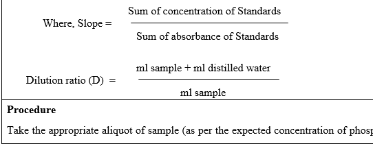
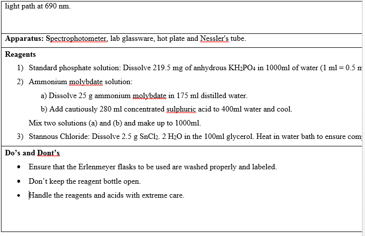
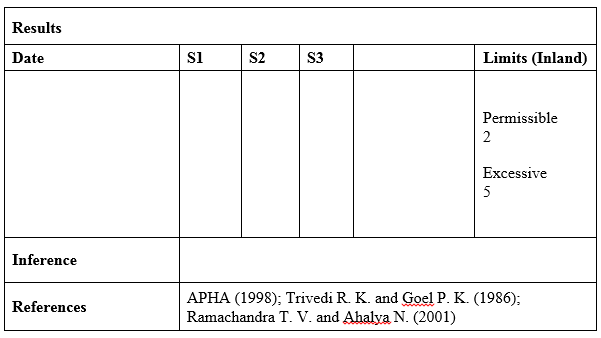
Table: Surface Water Quality Standards (as per IS: 2296).
Class A – Drinking water without conventional treatment but after disinfection. Class B –Water for outdoor bathing. Class C – Drinking water with conventional treatment followed by disinfection. Class D – Water for fish culture and wild life propagation. Class E – Water for irrigation, industrial cooling and controlled waste disposal. (Unobj = Unobjectionable).
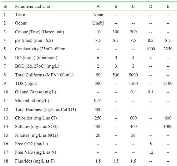
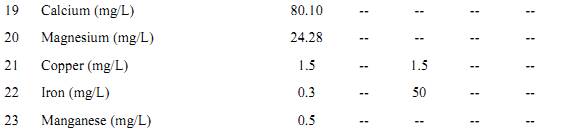
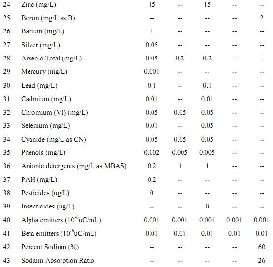
BIOLOGICAL PARAMETERS |
PLANKTON ANALYSIS: The physical and chemical characteristics of water affect the abundance, species composition, stability and productivity of the indigenous populations of aquatic organisms. The biological methods used for assessing water quality includes collection, counting and identification of aquatic organisms; biomass measurements; measurements of metabolic activity rates; toxicity tests; bioaccumulation; biomagnifications of pollutants; and processing and interpretation of biological data. The work involving plankton analysis would help in:
- Explaining the cause of colour and turbidity and the presence of objectionable odour, tastes and visible particles in waters.
- The interpretation of chemical analyses.
- Identifying the nature, extent and biological effects of pollution.
- Providing data on the status of an aquatic system on a regular basis.
|
Plankton:A microscopic community of plants (phytoplankton) and animals (zooplankton), found usually free floating, swimming with little or no resistance to water currents, suspended in water, non-motile or insufficiently motile to overcome transport by currents, are called "Plankton".
Phytoplankton (microscopic algae) usually occurs as unicellular, colonial or filamentous forms and is mostly photosynthetic and is grazed upon by the zooplankton (microscopic protozoans, rotifers, cladocerans and copepods) and other organisms occurring in the same environment.
The structure of photosynthetic populations in the aquatic ecosystems is dynamic and constantly changing in species composition and biomass distribution. An understanding of the community structure is dependent on the ability to understand the temporal distribution of the different species. Changes in species composition and biomass may affect photosynthetic rates, assimilation efficiencies, rates of nutrient utilization, grazing, etc.
Plankton, particularly phytoplankton, has long been used as indicators of water quality. Because of their short life spans, planktons respond quickly to environmental changes. They flourish both in highly eutrophic waters while a few others are very sensitive to organic and/or chemical wastes. Some species have also been associated with noxious blooms causing toxic conditions apart from the tastes and odour problems. |
Plankton net:The plankton net is a field-equipment used to trap plankton. It has a polyethylene filter of a defined mesh size and a graduated measuring jar attached to the other end. A handle holds the net. The mesh size of the net determines the size range of the plankton trapped. The mesh number 30 of size 60 mm was used for collecting samples. |
Sampling Procedure:The manner in which sampling is done should conform to the objectives of the study. The “surface samples” (samples collected from the surface) are collected as close to the water surface as possible, mostly towards the center of the lake at regular monthly intervals. A known volume of the sample, 5L to 50 L is filtered and planktons are filtered and preserved for further analysis. |
Labels:The sample label has the date, time of sampling, study area-lake name and the volume measured and pasted on the containers of 50 ml capacity. |
Preservation:The samples are collected into 100 ml polyethylene vials and are preserved by adding suitable amounts of 1ml chloroform to act as the narcotizing agent and 2 ml of 2% formalin for preservation and analyses. |
Concentration technique: The plankton nets are used to collect samples for the qualitative and quantitative estimation of the plankton, by filtering a known volume of water (5-50 liters) through the net depending on the plankton density of the tanks. |
Qualitative and quantitative evaluation of plankton:Detailed analyses of phytoplankton populations are done by estimating the numbers in each species. The phytoplankton consisting of individual cells, filaments and colonies are counted as individual cells. When colonies of species are counted, the average number of cells per colony is counted, and in filamentous algae, the average length of the filament has to be determined. |
Sedimentation and enumeration by microscope:Preserved samples in bottles are mixed uniformly by gentle inversion and then exactly 1ml of the sample is pipetted out into the S-C cell for analysis. |
Microscope
Compound microscope: A monocular compound microscope is used in the counting of plankton with different eyepieces such as 4X, 10X and 40X. The microscope is calibrated using plankton-counting squares. |
Counting
Counting cell- Sedgwick-Rafter (S-R) cell: The Sedgwick-Rafter cell is a devise used for plankton counting and is about 50mm long by 20mm wide and 1mm deep. The cell is covered by a relatively thick cover slip and is calibrated to contain exactly 1.0 ml.
Method
Filling the cell:The cover slip is placed diagonally across the S-R cell and filled with the sample carefully without air bubbles with a large bore pipette. The sample is allowed to settle for about 5 minutes before the actual counting begins. |
Note: Since the configuration of the S-R cell does not allow the use of high power microscope objectives, the identification of organisms smaller than 10 – 15 mm is difficult or impossible, limiting the usage to only larger forms of relatively dense populations.
Strip counting: A "strip" is the length of the cell that constitutes a volume approximately 50 mm long, 1-mm deep accounting to the volume of 25mm3 or 1/40 (2.5%) of the total cell volume. By moving the mechanical stage from left to right, the organisms can be examined in a systematic manner. By knowing the surface area of the portion counted in relation to that of the total, a factor is determined to expand the average counts of the plankton to the total area of the counting surface. This total area represents the number of organisms present per given volume of the sample. This volume expanded to an appropriate factor yields the organisms per litre of water for the lake.
The total number of planktons in the S-R cell is obtained by multiplying actual count in the strip by the number (enumeration factor) representing the portion of the S-R cell counted. The number of the strips counted is a function of the precision desired and the number of units (cells, colonies) for the strips measured. In this study, 500 cells were counted for estimation.
The plankton count in the S-R cell is got from the following,
C X 1000 mm
Number/ml = -------------------------
L X D X W X S
Where
C = Number of organisms counted
L = Length of each strip (S-R cell length) mm
D = Depth of a strip (S-R cell depth) mm
W = Width of a strip in mm
S = Number of strips counted
V1 = (50)(1)(W)
= mm3
The plankton counts per strip are then determined by multiplying the actual count by the factor representing the counted portion of the whole S-R cell volume.
Number/ml = (C) (1000 mm3) / (L) (D) (W) (S)
Where
C = Number of organisms counted.
L = Length of each strip in mm (of S-R cell)
D = Depth of the strip in mm (S-R cell)
W = Width of the strip in mm (Whipple grid image width)
S = Number of strips counted.
Phytoplankton Counting Units: Some plankton are unicellular while others are multicellular (colonial), posing a problem for enumeration. For analysis, a colony of plankton is accounted as a single count. The large forms that cross two or more boundaries of the grid are counted separately at lower magnification and their number included in the total count. |
COMMONLY FOUND ALGAL GROUPS IN LAKES |
Bacillariophytes: They occur in fresh water, salt water, and terrestrial ecosystems. They are single-celled algae with shells constructed of two overlapping valves composed of pectin and impregnated with silica. Amorphous silica is the form of silicon in diatom cell walls. The diatoms are single-celled or unicellular organisms, but some can form colonies and filaments. They may occur as plankton or periphyton, with most brownish-green films on substrates such as rocks or aquatic plants being composed of attached diatoms. The Bacillariophytes comprises two main types: centric and pennate. Centric diatoms are radially symmetrical and pennate diatoms that are bilaterally symmetrical. Many diatoms have conspicuous oil droplets within the cell, which is the photosynthetic food reserve, chrysolaminarin. The diatoms contain the pigments chlorophyll a and b, alpha and beta carotene, and several xanthophylls.
Example: Nitzschia sp., Cymbella sp., Melosira sp., Navicula sp., Gomphonema sp., Cyclotella sp., Pinnularia sp., Gyrosigma sp., etc. |
Euglenoids: Typically green and unicellular, euglenoid flagellates occur in most freshwater habitats: puddles, ditches, ponds, streams, lakes, and rivers, particularly waters contaminated by animal pollution or decaying organic matter. Most are photosynthetic, but many, lacking chloroplasts are heterotrophs. Most do not reproduce sexually. Euglenoids lack a cellulose cell wall; instead, they have a proteinaceous pellicle just inside the plasmalemma. Euglenoids are characterized by chlorophylls a, b, beta carotene, and xanthophylls, one membrane of chloroplast endoplasmic reticulum, a mesokaryotic nucleus, two emergent flagella with fibrillar hairs in one row and paramylon or chrysolaminarin as the storage product in the cytoplasm. They have eyespot (stigma) which is a collection of orange-red lipid droplets. If placed in the dark over the course of several divisions, the chloroplasts of Euglena gracilis will become colorless. When returned to the light, the plastid structure is reformed and the green color returns. All euglenoid species with an eyespot and flagellar swelling exhibit phototaxis, usually swimming away from bright light (negative phototaxis) and away from darkness toward subdued light (positive photoaxis) to accumulate in a region of low light intensity.
Example: Euglena sp., Phacus sp., Trachelomonas sp., etc. |
Blue-Green Algae (Cyanobacteria): The cyanophytes are the only prokaryotic algae and lack membrane bound organelles. Cyanobacteria are aerobic phototrophic organisms that can perform photosynthesis as they possess chlorophyll a and photosystem II. They are ubiquitous in nature and are found in every type of environment including terrestrial, freshwater, and marine habitats. Blue green algae are very common in waters of a great range of salinity and temperature, and they occur in and on the soil and also on rocks and in their fissures. However, the external structure can range from unicellular or colonial to branched or unbranched and filamentous. The cyanobacterial cells possess a number of cell inclusion bodies like include phycobilisomes, carboxysomes, glycogen granules, polyphosphate granules, poly-β –hydroxybutyrate granules, cyanophycin granules and gas vesicles. The cyanophytes possess no flagellated or cilliated cells at any stage of their lifecycle, although, simple movements such as bending and swaying are made possible by internal pressure changes exerted on the cell wall. They are heavily pigmented with chlorophyll a, beta carotene, and several xanthophylls. The presence of several phycobiliproteins gives the cyanophyta their unique blue-green coloration. Food is stored in the form of glycogen. Example: Microcystis sp., Merismopedia sp., Phormidium sp., Anabaena sp., etc. |
Green Algae (Chlorophytes): Chlorophytes are a diverse group and are common in fresh water, salt water, and soil. The chlorophyta are primarily freshwater; only about 10% of the algae are marine, whereas 90% are freshwater. Green algae have unicellular or multicellular thalli. Some are flagellates, and others produce reproductive cells, the majority of which are biflagellate. Chlorophyte reproduction varies greatly, from asexual division to isogamy and heterogamy to oogamy. Cell walls are constructed of cellulose and pectin. The food storage product is true starch, the same as plants. Green algae possess true chloroplasts, which contain the same pigments found in higher plants: chlorophyll a and b, alpha and beta carotene, and many xanthophylls.
Example: Chlorella sp., Ankistrodesmus sp., Chlamydomonas sp., Pandorina sp., Eudorina sp., Chlorogonium sp., Actinastrum sp., Pediastrum sp., Scenedesmus sp., etc. |
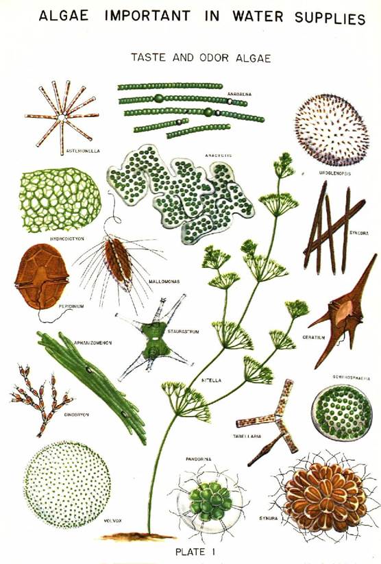
Citation: Ramachandra T V, Subash Chandran M D, Bharath Settur, Deepthi Hebbale, Prakash Mesta, Rajasri Ray, Sudarshan P. Bhat, Asulabha K S, Sincy Varghese, Durga Madhab Mahapatra, Harish R. Bhat, Vinay S,. Vishnu D Mukri,,Gouri Kulkarni, Bharath H. Aithal, 2016. My Village Biodiversity: Documentation of Western Ghats Biodiversity through Network of Students and Teachers, Sahyadri Conservation Series 61, ENVIS Technical Report 113, Environmental Information System, CES, Indian Institute of Science, Bangalore 560012
| | | |