Results

Landscape condition analysis

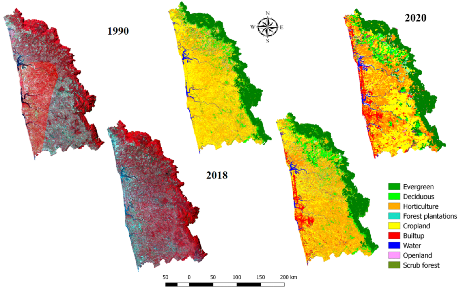
Spatiotemporal quantification of LU transitions in Udupi for 1990-2020 was performed using the Maximum Likelihood Classification algorithm and accuracy of the classified map was analyzed by estimating kappa value and overall accuracy. LU map of Udupi has been shown in Figure 3. The built-up area in the coastal region increases from 1485 hectares to 33,052.53 hectares, of 8.81% during the three decades. Area under forest cover i.e., evergreen and deciduous has decreased from 11.74%, 10.47% (1990) to 11.21%, 9.16% (2020) respectively. Scrub forest increased from 1.85% (1990) to 2.76% (2020). The conversion of agricultural land to commercial use along the major highways has increased the built-up area. Horticulture plantations increased from 36.86% to 43.77% with rubber plantations during three decades (Table 2).

Figure 3. LU analysis of Udupi from 1990 to 2020

Table 2. Land uses in Udupi District (1990-2020)

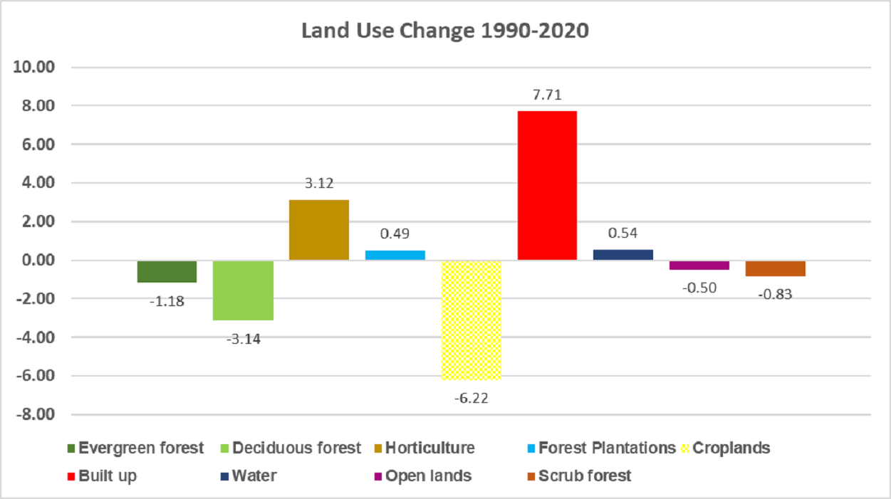
Figure 4, illustrates that scrub forest increase by 1.37%, and built-up areas increased by 7.17%. Horticulture plantations replace agricultural activities during three decades.

Figure 4. Percentage change in LU analysis of Udupi during (1990-2020)

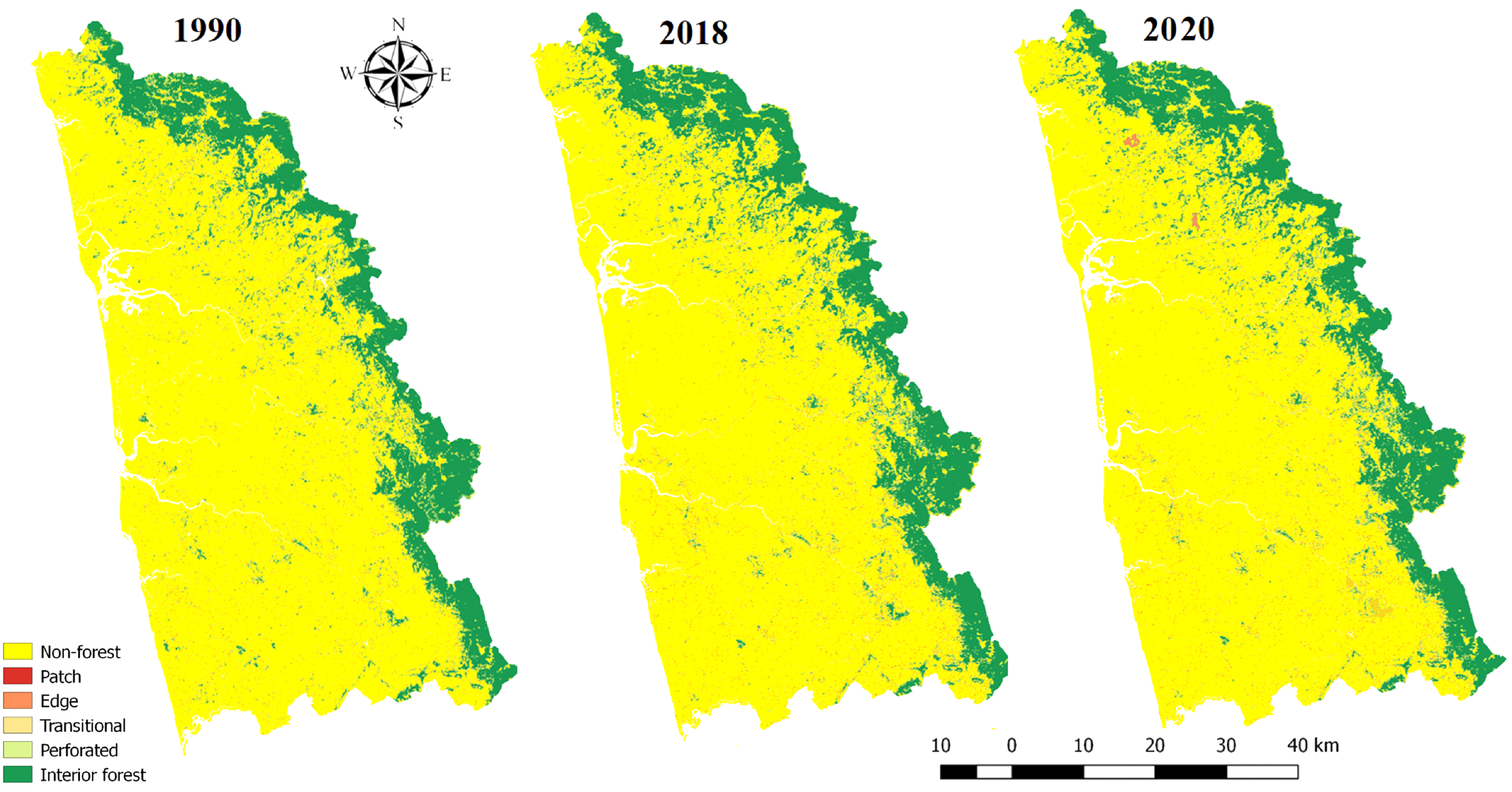
Fragmentation analyses show loss of intact forest (core),, and Figure 5 depictsfragmentation fromg 1990 to 2020. Table 3 gives the spatial extent of various types of fragments (interior non-forest, patch forest, transitional forest, edge forest, perforated forest, and interior forest). Area under interior forest has decreased from 16.77% (1990) to 13.97% (2020) while non-forest areas has increased from 74.27% (1990) to 78.24% (2020). The transitional forest has decreased from 1.8% (1990) to 1.04% (2020), with increased edge forests indicating the boundary between interior forest and non-forest has increased. The increase in non-forest areas signifies a major portion of the forest area has been converted into built-up areas, croplands, roads, etc. The core forest exists only as protected areas, sanctuaries, national parks, and sacred groves.

Table 3. Fragmentation Analysis of Udupi District (1990-2020)

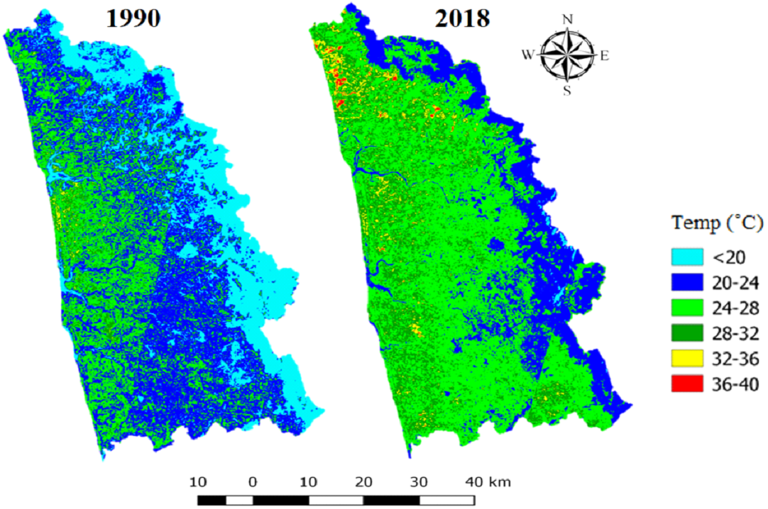
Land Surface Temperature [LST]

The higher temperature can be seen especially in non-forest areas due to an increase in built-up areas. The temporal LST analysis shows hilly regions are with moderate surface temperatures, evident from Table 4. Urban areas show an increase in temperature (maximum) from 30.71˚C (in 1990) to 37.51 ˚C (in 2018). Due to a reduction in the interior or intact forest cover, there is an increase in temperature from 29.47 ˚C (in 1990) to 38.94 ˚C (in 2018). Table 4 also illustrates the change in temperature across land-use categories over the period. The maximum change in temperature was observed over forest cover (with the fragmentation of forests) by 6.39 ˚C followed by non-forest cover by 5.70 ˚C during the past 28 years, comparable with ground data.

Table 4. Temperature Analysis of Udupi District (1990-2018)

Figure 5. Temporal dynamics of LST of Udupi from 1990-2018

Conservation Importance Regions (CIR)

Compilation of attribute data related to ecology, geo-climate, land, and social aspects has been collected, and aggregated weight has been computed.

Ecology

The ecosystem's health is assessed based on key variables such as conservation status, diversity, etc. Data is compiled from the field, review of published literature, and virtual data portals (such as avibase, ifoundbutterflies, etc.). Conservation Reserves (CR) have been established under Protected Areas under the Wildlife Amendment Act of 2002. Conservation Reserves are essentially the buffer zone between National Parks (NP), Wildlife Sanctuaries, and reserve forests. 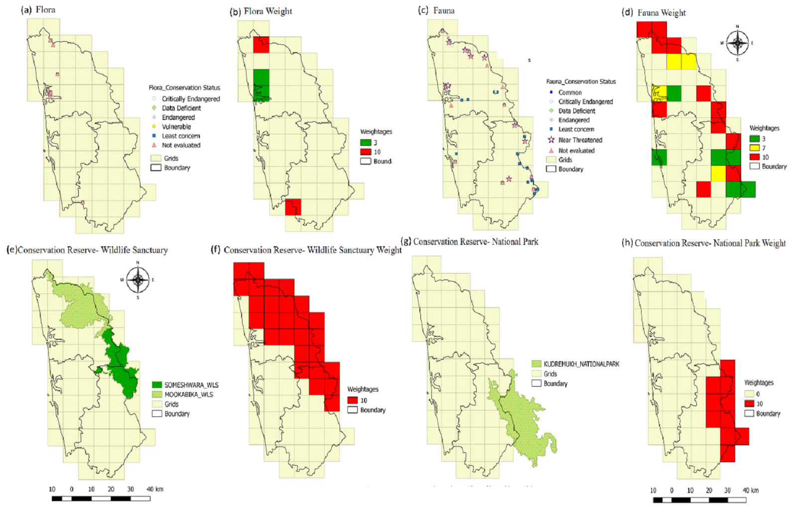Higher weights were assigned to CR and NP, and the grids with the critically endangered and endangered species were assigned a value of 10, vulnerable and near-threatened species are assigned a value of 7, threatened species is assigned 5, common, data deficient, rare and lower risk were assigned a value of 3 while not evaluated is assigned a value of 1. Figure 6a-h depicts the distribution of flora and fauna with conservation status and weights, which shows most of the species are concentrated across wildlife sanctuaries in the district.

Figure 6. Ecological variables with their weights

The flora of Udupi district has been compiled by reviewing published literature and data portals. The district is home to critically endangered species such as Elaeocarpus gaussenii, Syzygium travancoricum, Utleria salicifolia, Vateria indica, Vatica chinensis and vulnerable species such as Chloroxylon swietenia, Cinnamomum sulphuratum, Dalbergia latifolia, Garcinia indica, Myristica malabarica, Ochreinauclea missionis, Paracautleya bhatii, Santalum album, Saraca asoca, Saraca indica. The dominant families are Fabaceae, Lamiaceae, Dipterocarpaceae, Euphorbiaceae.

Udupi district has rich faunal diversity. The region has near-threatened amphibian species such as Philautus beddomii, Ramanella montana, Rana curtipes, Tomoptema rufescens, and vulnerable species such as Ichthyophis beddomei, Micrixalus Saxicola, Nyctibatrachus major, Philautus glandulosus, Rana aurantiaca, Rana leithi. Mammals species such as Bos gaurus, Cervus unicolor, Funambulus subineatus, Melursus ursinus, Neophocaena phocaenoides, Physeter macrocephalus are under near threatened and species are Hyaena hyaena, Lutra lutra, Panthera pardus, Ratufa macroura, Sousa chinensis under vulnerable category of IUCN conservation status. The district has critically endangered birds such as Fregata andrewsi, Gyps bengalensis, Gyps indicus, Sarcogyps calvus and vulnerable category birds such as Chaetornis striata, Ciconia episcopus, Clanga clanga, Clanga hastata, Columba elphinstonii, Gallinago nemoricola, Leptoptilos javanicus, Schoenicola platyurus. The district has vulnerable category reptiles such as Cnemaspis indica, Cnemaspis indraneildasi, Cnemaspis jerdonii, Hemidactylus albofasciatus, Hemidactylus sataraensis, Kaestlea laterimaculata, Melanophidium bilineatum, Oligodon brevicauda, Uropeltis phipsonii

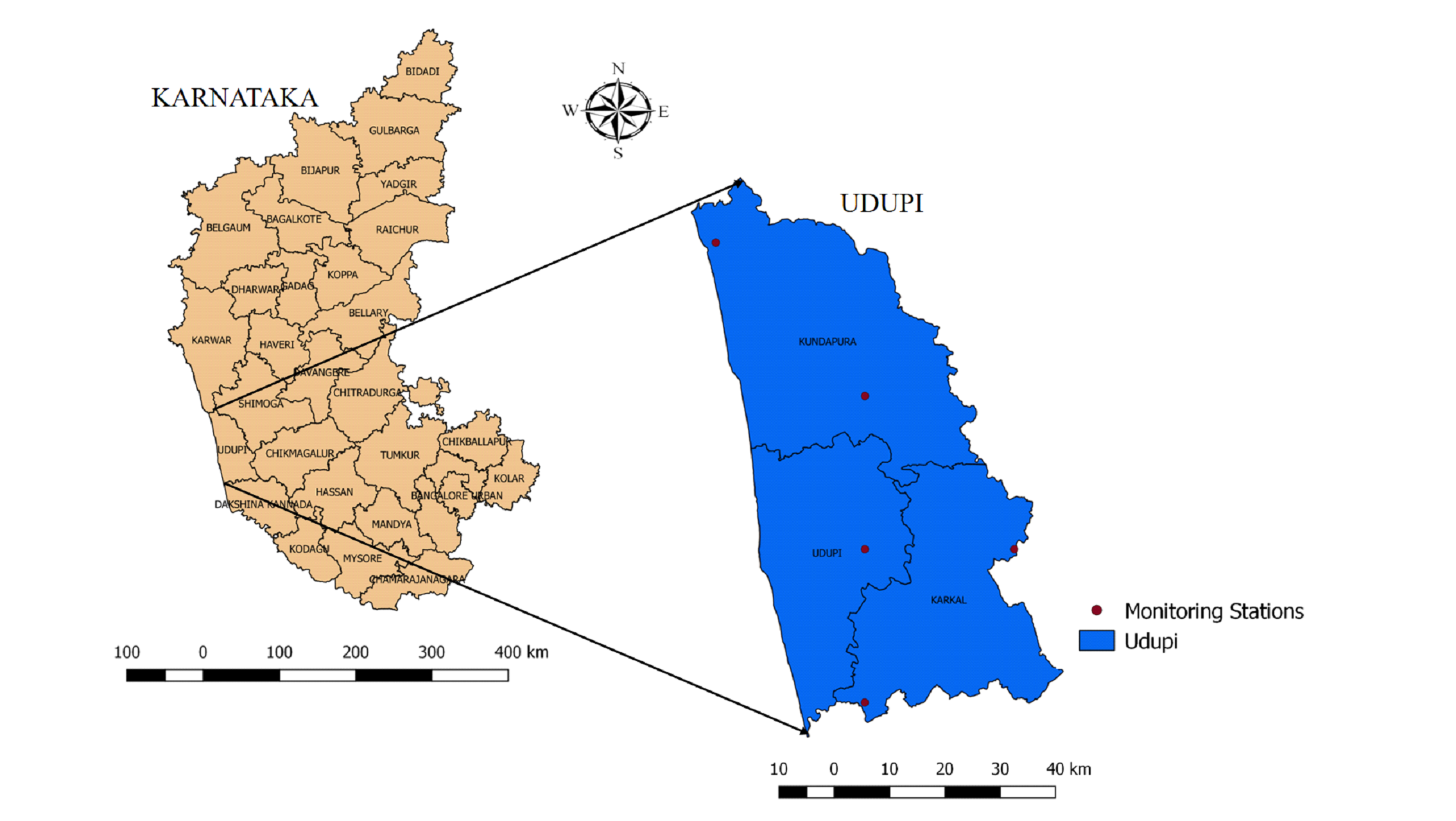
Kudermukh National Park covers a minor portion of the study region and shares its boundary with Dakshina Kannada. The study region has diverse flora and fauna: 162 species of flowering plants representing 50 families. Fabaceae had maximum tree species (23), followed by Rhizophoraceae (17 species), Moraceae (7 species) – known as the family of figs and keystone species for plants, etc. Vateria indica is one of the critically endangered species present in the district while Hopea ponga, and Syzygium caryophyllatum are the two endangered species, and Garcinia indica, and Ochreinauclea missionis are the two vulnerable species that are well distributed in the district. Someshwara and Mookambika wildlife sanctuary are known for the variety of birds and wild flowering species endemic to the region. 816 species of fauna representing 123 families were documented. Malabar Grey Hornbill, Small Green Barbet, Gotyla, Rock Bush Quail, Grey Jungle fowl, Malabar Wood shrike, Indian Rufous Babbler, Nilgiri Thrush, Nilgiri Blue Robin, Day's GlassFish, Gunther's catfish, Tyler’s Leaf Warbler, etc., are found in the district.

Geo-climate

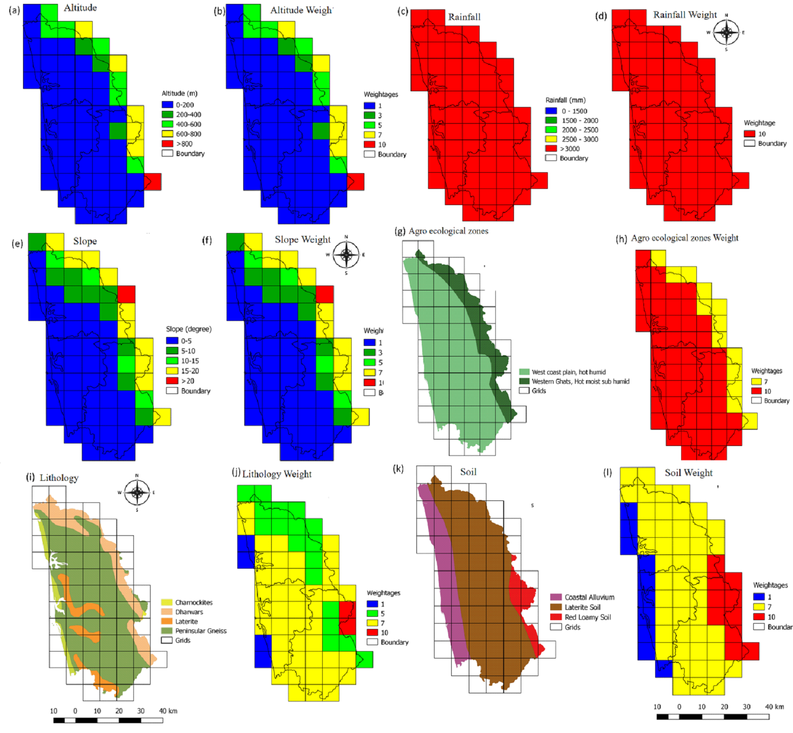
The geo-climatic parameter plays a crucial role in determining the landscape dynamics of any region. Figure 7a-l depicts the different geo-climatic parameters in the region and their weights assigned to the grids. The patterns of altitude, slope, rainfall helps in determining the forest cover, biodiversity, etc., of a region. The rainfall pattern shows entire district receives high rainfall during all seasons. The coastal part falls under a hot moist sub-humid region can be attributed to a favorable climatic pattern for healthy vegetation. Grids with high rainfall and soil types have rich forest cover with high biodiversity and conservation values. Regions with high rainfall, elevation, and slope were assigned a value of 10, and the lowest is given a value of 1. Loamy soil is considered best for agricultural purposes with rich porosity and humus content, which is assigned a value of 10, while laterite and mixed red and black soil are assigned a value of 7, red sandy and medium black were given 5 and coastal alluvium as 1. Lithology is an important factor considering landscape structure and patterns. Charnockites was given the highest value of 10 followed by peninsular gneiss of 7, closepet granite, and Dharwars were assigned 5 while alluvium was assigned 1. Agro-ecological zones play a significant role in determining the climate of a region. Therefore, hot humid is assigned the highest value of 10 as the region receives high rainfall around 1500mm or more. Hot moist sub-humid is assigned 7, hot dry sub-humid is given 5, and hot moist semi-arid is assigned the lowest value of 3.

Figure 7. Geo-climatic factors and their weight

Land

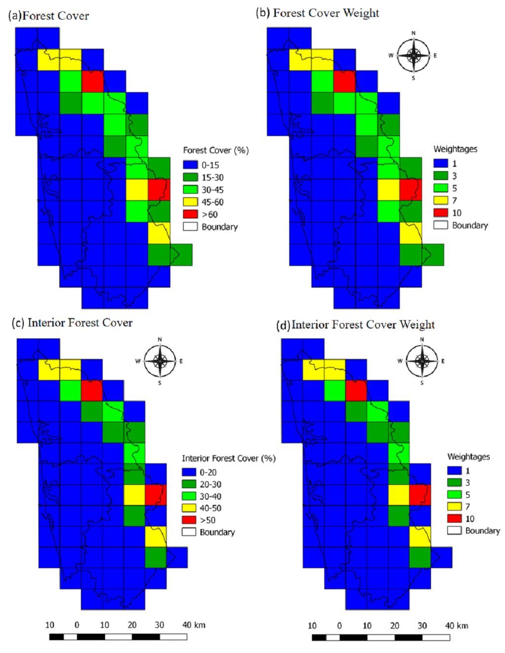
Grids are prioritized based on the proportion of forest cover. Forest fragments were computed using standard protocol wherein interior core forest patches were considered devoid of any edge effects. Grids having more than 60% forest cover were assigned a value of 10, and accordingly, values were assigned. Land use analysis revealed that the region has about 2.98% under evergreen forest. Most parts are with less than 15% forest cover. Expansion of agricultural activities and the introduction of exotic species has led to the destruction of large forest patches at a temporal scale. The coastal taluks have a forest cover of less than 15% forest cover. Figure 8 depicts the weights assigned to the grids based on the extent of forest cover. Fragmentation analysis revealed that 3.39% of the area is under core interior forest while 94.25% area is under non-forest cover.

Figure 8. Land condition factors and weight

Social

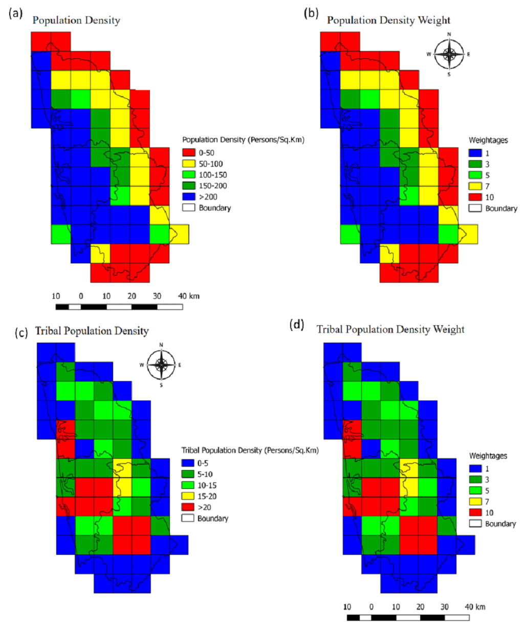
Population increase often leads to degradation of natural resources. An increase in population density will lead to loss of natural resources, species extinction etc. In this study, population density per sq. km has been considered as one of the influencing factors in resource use. Therefore, grids with less population density were given higher weights. Grid-wise, village population was computed for 2011. The grids with a population density of less than 50 persons were assigned high weights and vice-versa. Figure 9 depicts the population density assigned to the grids with corresponding weights. The hilly regions have high forest cover with less population density. Forest dwellers (tribes) of the study regions were mapped, and the grids with a high tribal population were given higher weight. Forest dwellers were spatially mapped and were given higher weights as they are directly or indirectly dependent on forest resources and also protect the forest.

Figure 9. Social factors considered and weight

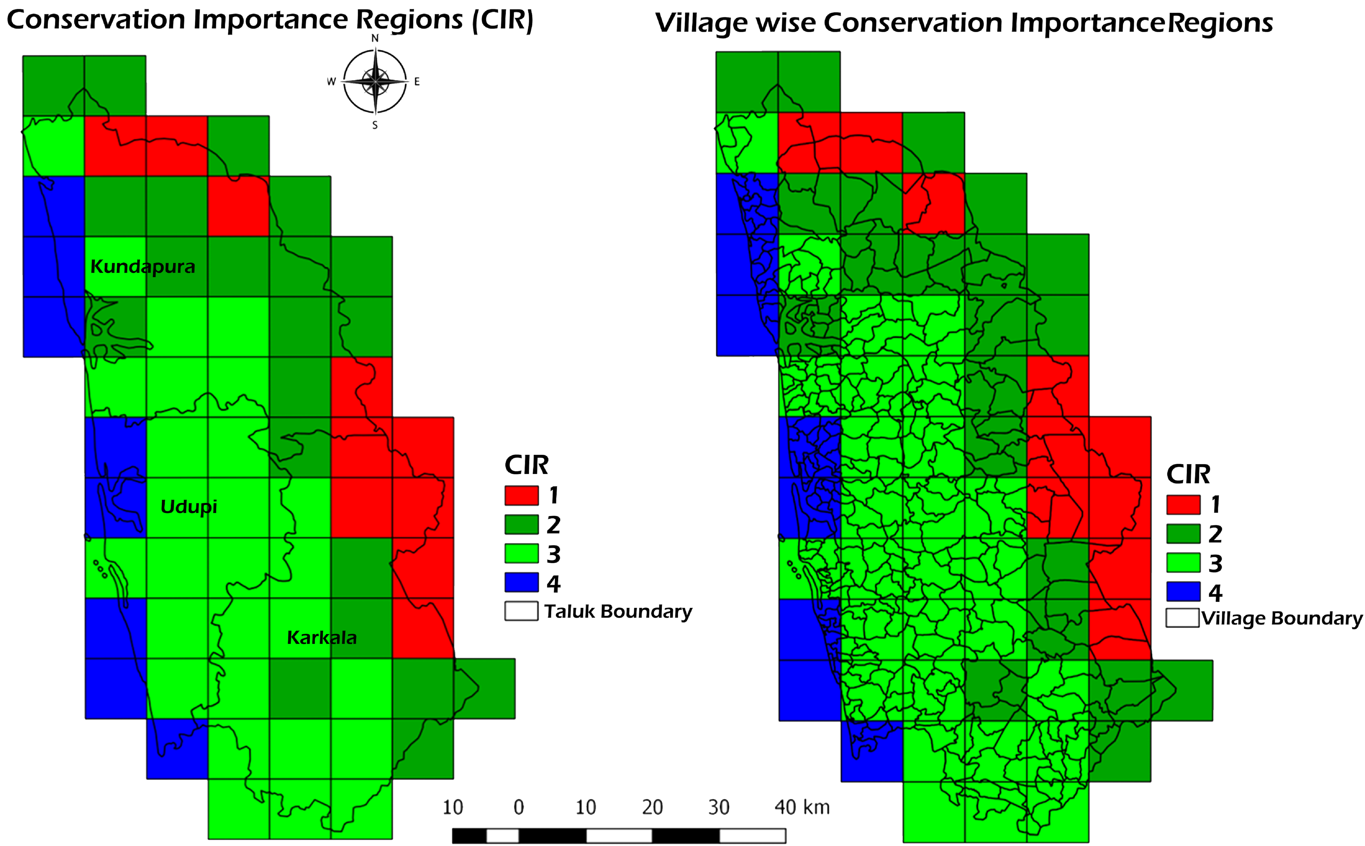
Based on the relative significance of themes, regions were prioritized using weightage metric score as CIR 1 (Regions of highest sensitivity), CIR 2 (Regions of higher sensitivity), CIR 3 (Regions of high sensitivity), and CIR 4 (Regions of moderate sensitivity). Spatially 15% of the district represents CIR1, while 31% of the area represents CIR2. 42% of the district represents CIR 3, and about 12% of the district is in CIR 4. Figure 10 depicts with taluk and village boundaries. CIR analysis at the village level shows only 14 villages in CIR 1, 52 villages in CIR 2, 178 villages in CIR 3, and 51 in CIR 4 (Figure 10) .

Figure 10. CIR at taluk and village level- Udupi District

LST in conservation importance region (ecologically sensitive regions)

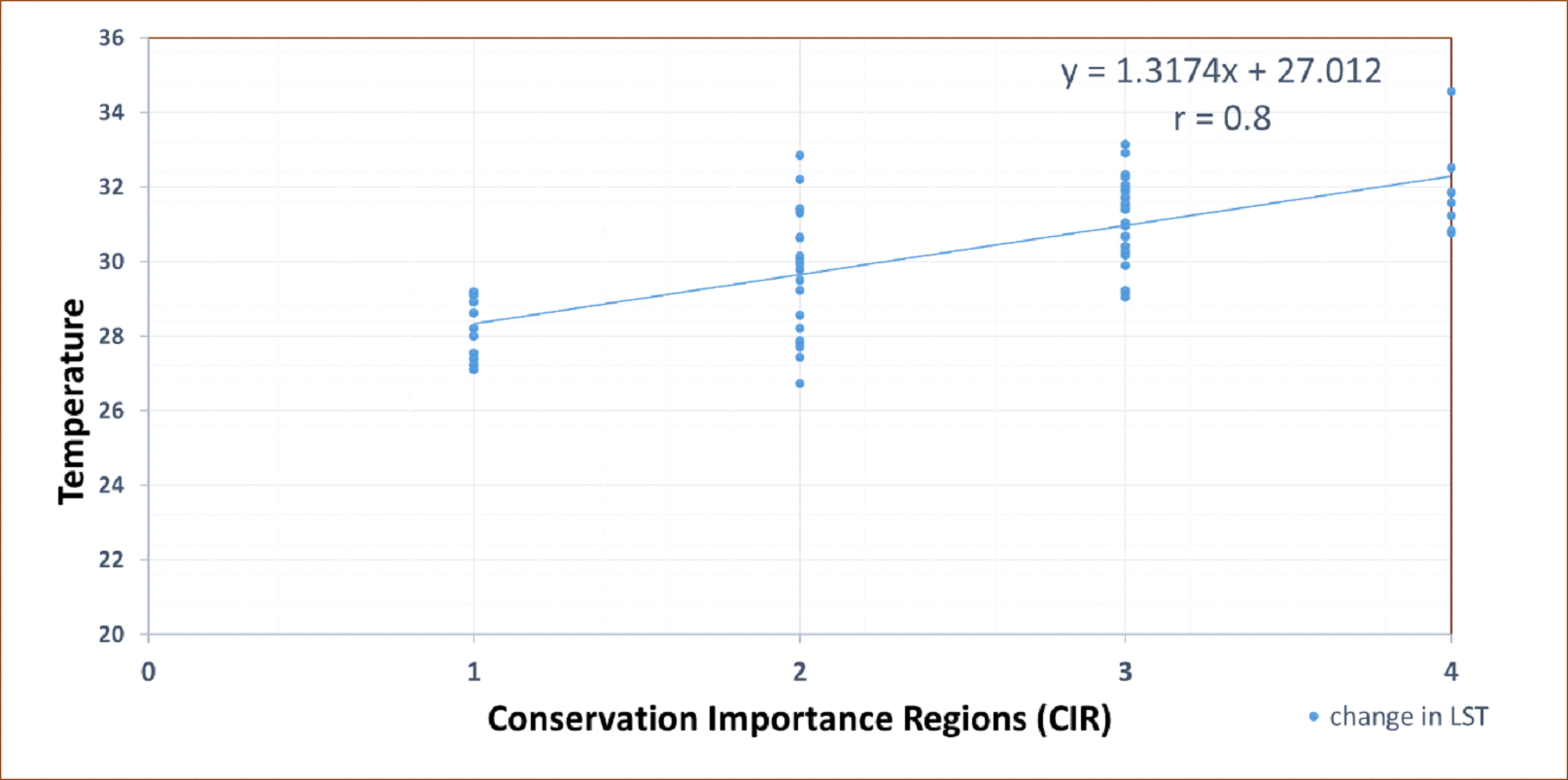
The ecological sensitiveness of a region has a direct impact on temperature. CIR 1has a lower temperature compared to CIR 2 -4. CIR 1 has the maximum forest cover and rich biodiversity along with less population, which aided in the low LST. LST trend shows an increase in temperature (r=0.8) across CIRs (Figure 11).

Fig. 11: Social factors considered and weight

Fig. 12: CIR at taluk and village level- Udupi District

Figure 13. LST across CIR- Udupi

Multivariate analysis is carried out to determine the relationship between LST and various independent variables (rainfall, forest cover, interior forest cover, and population density). In the study, variables considered are rainfall weight (x₁), forest cover (x₂), interior forest cover (x₃), and population density weight (x₄) to understand the change of temperature across the CIR regions in the districts. The probable relationship is given by

LST = 0 x₁- 0.28x₂ + 0.16 x₃ - 0.28 x₄+31.94 (r: 0.851, p <0.05)