Materials and Method

Study area

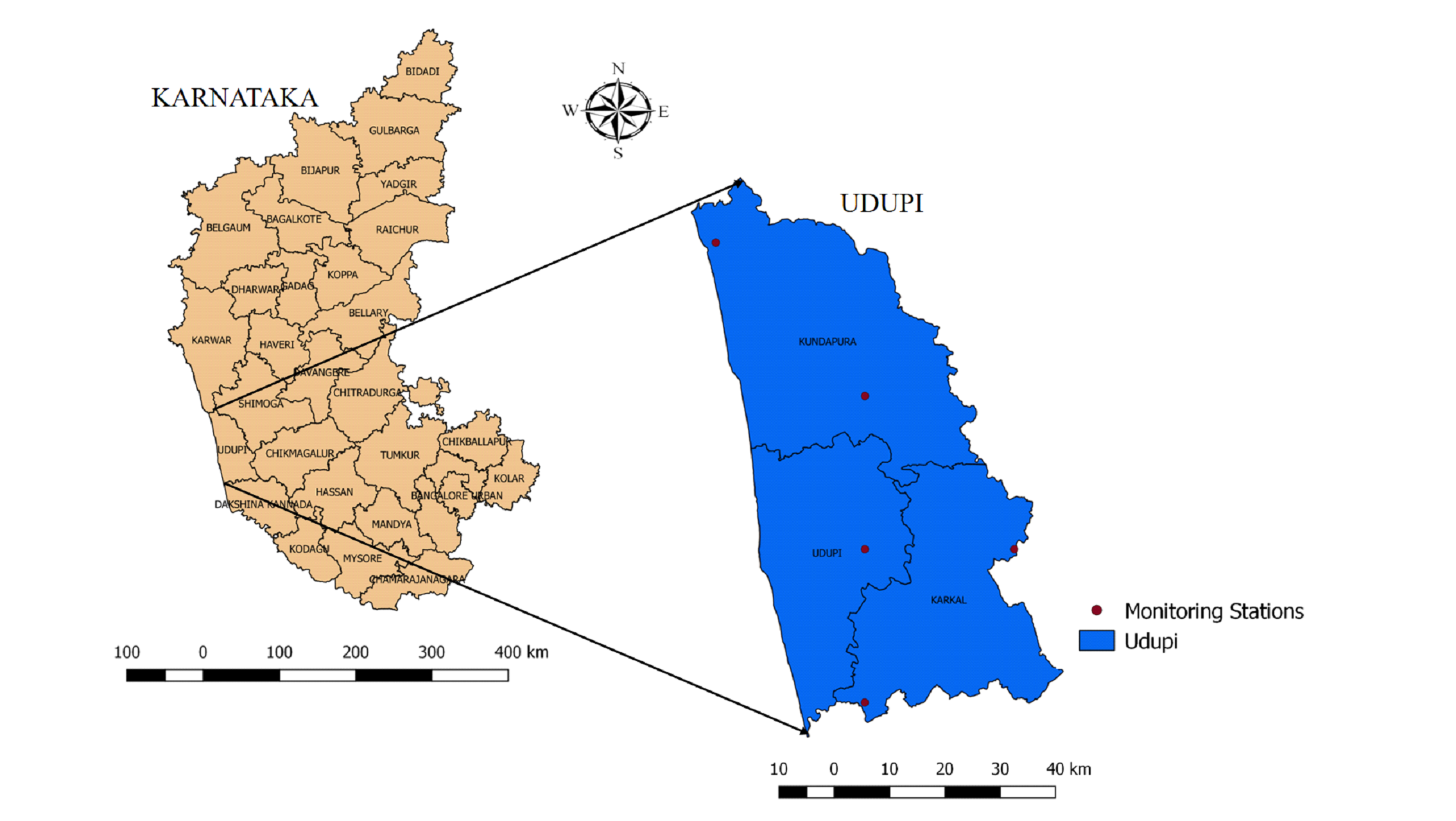
Udupi district (13°04' and 13°59' N latitude and 74°35' and 75°12' E longitude) was formed in the year 1997 with three taluks i.e., Udupi, Kundapur, and Karkala from the undivided parent district of Dakshina Kannada. The district is bounded by Uttara Kannada district in north and Dakshina Kannada district in southern direction with 3582 square kilometers geographical area (Figure 1). The district is blessed with abundant rainfall, fertile soil, and lush vegetation. The slopes of the Western Ghats are endowed with dense forests containing valuable species, including timber and fuelwood. The soils of the district are drained by perennial rivers such as Varahi, Gangolli, Sitandi, and Swarna, which join the Arabian Sea, known for its estuarine diversity. Udupi district gets an annual rainfall of 4000 mm. The climate is marked by heavy rainfall, high humidity, and sticky weather in the hot seasons. Pristine beaches, picturesque mountain ranges, temple towns, and rich culture make it a famous tourist destination. It is well known for Yakshagana- a fabulous costumed dance-drama form, Kambala- the buffalo racing sport by farmers, Kori-Katta (Cock Fight), and Bootha Kola. The district has witnessed largescale developmental activities post-2000 (Ramachandra and Aithal 2012).

Figure 1. Geographic location-Udupi District

Data

Spatiotemporal cloud-free remote sensing data of Landsat sensors (1990-2020) has been downloaded from the USGS-Earth explorer data portal. The Landsat data (all bands including the thermal band) were geo-registered to a common Universal Transverse Mercator coordinate system and resampled to 30 m using the nearest neighbour algorithm. Field data for LU classification and validation is collected using a pre-calibrated Global Positioning System (GPS). The data from Google Earth for various classes like forest, plantation, agriculture, urban, water and open spaces were also collected and used during analysis and validation. The temperature data of 2018 was taken from KSNDMC (Karnataka State Natural Disaster Monitoring Centre), used for LST validation. Global air temperature data (at 2 m from ground-based on climate modeling grid of 0.25) is used to validate LST maps for 1990. A 10 km daily meteorological dataset of 0.25 deg grid is used to validate LST of 1990. The dataset is based on the NCEP‐NCAR reanalysis (https://psl.noaa.gov/data/gridded /data.ncep.reanalysis.pressure.html#) merged with the University of East Anglia Climate Research Unit (CRU) monthly gridded temperature product and the NASA Langley Surface Radiation Budget (SRB- https://asdc.larc.nasa.gov/ project/SRB) product and the data are available in ‘NetCDF’ format with one file per variable per year. Population data of 1901, 2001, and 2011 were collected from the Census of India (https://censusindia.gov.in/). Geological data such as soil, lithology, and agro-ecological zones were obtained from ICAR- NBSS & LUP (National Bureau of Soil Survey and Land Use Planning). Elevation data was obtained from USGS EROS Archive - Shuttle Radar Topography Mission (SRTM) of 30-meter resolution. Terrain analysis was carried out for obtaining slope. Rainfall data is obtained from WorldClim- Global Climate Data version-2 (gridded climate data) with a spatial resolution of about 1 km².

Method

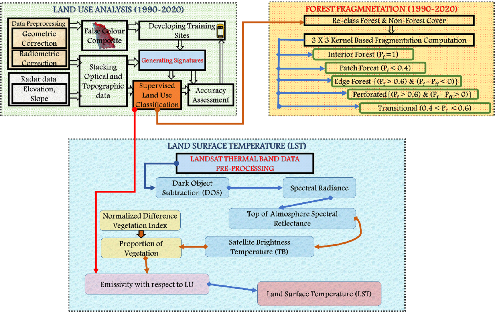
The present study has been carried out in three phases (i) using remote sensing data to analyse forest ecosystem extent and conditions (fragmentation), (ii) identify and prioritize conservation importance regions or ecologically sensitive regions based on ecology, geo-climatic, land, and social attributes, (iii) quantifying LST and evaluating the relationship between CIR and LST.

LU analysis involved,

1. Quality parameters: The remote sensing data were chosen to be devoid of or minimal cloud cover (less than 10 percent) and pixel quality.
2. Image pre-processing and geo-referencing: The data was rectified radiometric errors and geometric errors. Geometric rectification is done using ground control points with the nearest neighborhood technique. The geo-rectified image is then projected to WGS/UTM 43N (EPSG: 32643).
3. LU Classification: Remote sensing data is classified using a supervised classifier based on the Gaussian Maximum Likelihood algorithm. In the supervised technique, training data of representative LU describing the spectral attributes (Lillesand et al. 2014) is considered. The technique essentially considers variance and covariance of unknown pixels (Reddy 2009; Ganasri and Dwarakish 2015; Ramachandra and Bharath 2019b).
4. Validation of LU information: Classified LU information is validated by accuracy assessment through computation of error matrix and Kappa statistics. Error matrix compares, on a category-by-category basis, the relationship between ground truth data (reference data) and the corresponding results of the classified data. Kappa coefficient measures the difference between the actual agreement between the reference data and classified data and is estimated through equation 1.

Evaluating ecosystem condition:

The condition of the forest ecosystem is assessed through fragmentation analyses involving both the extent of the forest and its spatial pattern. Fragmentation of forests measures the degree to which forested areas are broken into smaller patches and pierced with non-forest cover. It is estimated through the computation of P_f and P_ff. P_f is the ratio of the number of pixels that are forested to the total number of non-forested non-water pixels in the kernel (3 × 3) and P_ff is the proportion of all adjacent (in all cardinal directions) pixel pairs that include at least one forest pixel, for which both pixels are forested. Various levels of fragmentation consist of five components: (i) Interior forest: It is essentially consisting of thick forest cover, (ii) Patch forest: Forest area comprising small forested areas surrounded by non-forested land cover, (iii) Perforated forest: Forest pixels forming the boundary between an interior forest and relatively small clearings (perforations) within forest landscape, (iv) Edge forest: Forest pixels that define the boundary between interior forest and large non-forested land cover features and (v) Transitional forest: Areas between edge type and non-forest types. If higher pixels are non-forest, they will be tending to non-forest cover with a higher degree of edge.

Figure 2. Method adopted for LU, fragmentation, and LST analysis

Land Surface Temperature [LST] estimation

LST is estimated using time series data from top-of-atmosphere brightness temperatures from the infrared spectral channels of a constellation of geostationary satellites. Its estimation depends on the albedo, vegetation cover, and soil moisture (Bharath et al. 2013; Ibrahim et al. 2016; Sahana et al. 2016). LST influences the partition of energy between ground and vegetation and determines the surface air temperature. Retrieval of LST from Landsat 8 thermal data involves computation of radiance correction, reflectance correction, converting DN value to brightness temperature, computation of NDVI, the proportion of vegetation. Emissivity-corrected LST as follows:

L_λis TOA (temperature of atmosphere) spectral radiance (Watts/ (m² * srad * μm)), is Band specific multiplicative rescaling factor from the metadata, is Band specific additive rescaling factor from the metadata, is Quantized and calibrated standard product pixel values (DN).

Reflectance correctness ρλ′ = Mρ + Aρ 3

ρλ’ is TOA (temperature of the atmosphere) planetary reflectance, Mρ is Band-specific multiplicative rescaling factor from the metadata, Aρ is Band-specific additive rescaling factor from the metadata.

DN value converted to brightness temperature T_b = K₂ / ln [(K₁/L₁₀)+1] ... (4)

L10 is the spectral radiance of thermal band 10 [Wm−2sr−1μm−1], is the brightness temperature [Kelvin] and K 1 and K 2 are constants [Wm−2ster−1μm−1], K 1 = 666.09, K2 = 1282.71. Calculation of NDVI and Proportion of vegetation (P_v) using equations 5 and 6, respectively.

NDVI = Band5 - Band4 / Band5 + Band4 .... (5)

Where Band5 is the near-infrared band and band4 is the red band.

P_v = [NDVI-NDVImin/NDVImax-NDVImin]² .... (6)

Land surface emissivity is very important for calculating LST as it is the proportionality factor that scales blackbody radiance (Planck’s law) to predict emitted radiance, and it is the efficiency of transmitting thermal energy across the surface into the atmosphere (Kumari et al. 2018). Emissivity is very close to 1 for all objects, but to get a precise temperature, emissivity values for each LC class is separately considered (Table 1). The land surface emissivity LSE (ε) is calculated as proposed by Sobrino et al., 2004

ε = 0.004Pv + 0.986 .... (7)

where ε is the emissivity.

Table 1. Table showing LU categories and emissivity values

Emissivity-corrected LST in degrees Celsius T_b = [T_b/{1+[(λTb/ρ)lnελ]} ... (8)

ρ = h 1.438*10^-2 mK Where σ is the Stefan-Boltzmann constant (1.38*10−23J/K), h is the Planck's constant (6.626*10−32Js), and c is the velocity of light (2.998*108m/s).

Retrieval of LST from Landsat TM is as follows,

Radiance correctness L_λ = (Lmax - Lmin/Qcal_max - Qcal_min)*(Qcal - Qcalmin) + Lmin ... (9)

L_λ is temperature of atmosphere spectral radiance

Qcal is the quantized and calibrated standard product pixel value (DN)

DN value converted to brightness temperature T_b = [K_b/ln[(K₁/L_λ)+1] ... (10)

is the spectral radiance of thermal band 6 [Wm−2sr−1μm−1], is the brightness temperature [Kelvin] and K 1 a d K 2 are constants [mW*cm-2* sr-1], K 1 = 1260.56, K2 = 607.76. Emissivity corrected final LST will be computed using equation 7.

Prioritization of Conservation Importance Regions (CIR)

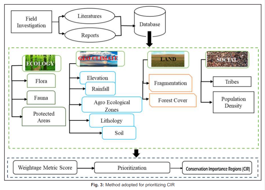
CIR refers to the areas of high ecological significance value. These are the regions where anthropogenic activities can cause alterations in the natural structure of the biological communities and natural habitats. The steps followed during identification and prioritization of CIR are detailed in Figure 2 and listed below:

1. Creation of grids: The study area is divided into grids of 5’ X 5’ covering approximately 9 X 9 km² (comparable to grids of the Survey of India topographic maps of scale 1:50000) for prioritizing CIR at decentralized levels (panchayat level).
2. Integration of data with grid: In this study, four different attributes being ecology, geo-climatic, land, and social were selected for the prioritization of CIR. Ecology consists of flora and fauna present in the region. Geo-climatic parameters refer to the various geological and climatic parameters such as rainfall, elevation, slope, LST, soil, agro-ecological zones, and lithology. Finally, land essentially consists of forest cover and interior forest extent and social, composed of tribal and social population density.
3. Weightage metric score: Weightages were assigned to attributes based on their significance value. The weightage metric score is estimated using equation 11.

Weightage = ∑i=1 WiVi

Where n is the number of data sets (variables), is the value associated with criterion i, and is the weight associated with that criterion. Based on the weightage, rank is given between 1 to 10 wherein value 10 corresponds to the highest priority for conservation, 7, 5, and 3 corresponds to high, moderate, and low level of prioritization, whereas 1 corresponds to least priority for conservation

1. Prioritization of CIR: Weights are aggregated for each grid and grouped into four groups as CIR 1, CIR 2, CIR 3 and CIR 4 based on the aggregated scores (CIR 1: aggregated scores > µ+2σ, CIR 2 (for grids within µ+2σ and µ+σ), CIR 3 (for grids with µ+σ and µ) and CIR 4 (grids with values < µ). In particular, the weightages are based on an individual proxy and depends extensively on GIS techniques, which is the most effective method.