|
Materials and Method
Study area: Uttara Kannada district lies between 13°55' to 15°31'N and 74°9' to 75°10'Espread over an area of 10,293 km2 in the mid-western part of Karnataka state, India (Figure 1). It is a region of gentle undulating hills, rising steeply from a narrow coastal strip bordering the Arabian Sea to a plateau at an altitude of 500 m with occasional hills rising above 600–860 m [33]. The district has 11 taluks covering three different zones i.e. coastal lands (Karwar, Ankola, Kumta, Honnavar and Bhatkal taluks), Sahyadrian interior (Supa, Yellapur, Sirsi and Siddapur taluks) and the eastern margin plains (Haliyal, Yellapur and Mundgod taluks). Uttara Kannada District has unique distinction of having different agro climatic zones and soil types. Coastal alluvial, Laterite are major soil types. According to 2011 census the ppopulation of district is 14, 36, 847 and population density is 140 persons per sq. km. From early 80’s the region is started experiencing changes in land use due to the developmental activities. This conversion has occurred largely at the expense of forests and grassland [34]. Major Industrial Infrastructure of this region constitutes 8 Industrial Estates & 1 Industrial Area.
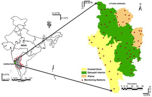
Figure 1: Study area - Uttara Kannada District
Method: Figure 2 outlines the procedure adopted in the current study. Data used in the study includes Landsat Thematic Mapper [TM] (March months of 1989, 1999), Landsat Enhanced Thematic Mapper plus [ETM+] (March 2009), and Google Earth (http://earth.google.com). The Survey of India topographic maps of 1:50,000 scales are used to generate base layers. The temporal remote sensing data of Landsat satellite were downloaded from the public domain (http://www.landsat.org) and geometrically corrected for the UTM coordinate system of zone 43 using GCPs (ground control points).Data are cloud free in March, transitional month from winter to summer. There are 3 India meteorological departments in the district which aided as validation stations apart from 80 locations of NOAA (http://neo.sci.gsfc.nasa.gov/Search.html) which are well distributed and cover whole district. Field data were collected using pre-calibrated handheld Garmin GPS. The study region has vast expanse of forests, training data is collected for different forest types and other land use categories. Theland cover analysis was done to assess the extent of area under vegetation, which is done through NDVI. Temporal normalised vegetation index (NDVI) is computed to assess the status of vegetation in the district. Among many indices, NDVI is most widely accepted for land cover analysis in the region dominated by vegetation cover [35, 36]. NDVI is computedby using visible Red (0.0.63 – 0.69 μm) and NIR (0.76 – 0.90 μm) bands of Landsat TM. Healthy vegetation absorbs most of the visible light that hits it, and reflects a large portion of the near-infrared light. Sparse vegetation reflects more visible light and less near-infrared light. NDVI ranges from minus one (-1) to plus one (+1). NDVI was calculated using Eq. (1). NDVI values range from -1 to +1 and very low values of NDVI (-0.1 and below) correspond to soil or barren areas of rock, sand, or urban built up. Zero indicates water cover. Moderate values represent low density vegetation (0.1 to 0.3), while high values indicate thick canopied vegetation (0.6 to 0.8).
 . . . (Equation 1) . . . (Equation 1)
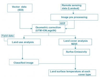
Figure 2: Method followed for LULC and LST analysis
Land use analysis involves i) generation of False Colour Composite (FCC) of remote sensing data (bands – green, red and NIR). This helped in locating heterogeneous patches in the landscape ii) selection of training polygons (these correspond to heterogeneous patches in FCC) covering 15% of the study area and uniformly distributed over the entire study area, iii) loading these training polygons co-ordinates into pre-calibrated GPS, iv) collection of the corresponding attribute data (land use types) for these polygons from the field. GPS helped in locating respective training polygons in the field, v) supplementing this information with Google Earth (http://googleearth.com) and Bhuvan (http://bhuvan.nrsc.gov.in), vi) 60% of the training data has been used for classification, while the balance is used for validation or accuracy assessment.
Land use analysis was carried out using supervised pattern classifier - Gaussian Maximum Likelihood Classifier (GMLC) algorithm. Remote sensing data was classified using signatures from training sites that include predominant land use types. Mean and covariance matrix are computed using estimate of maximum likelihood estimator. This technique is proved to be a superior classifier as it uses various classification decisions using probability and cost functions [37]. GRASS (Geographical Analysis Support System) a free and open source software having robust support of processing both vector, raster files has been used for this analysis. GRASS is freely accessible and downloadable at http://wgbis.ces.iisc.ac.in/grass/index.php.The images were maintained at common resolution of 30m by downscaling. Downscaling is the enhancement of the spatial resolution of the original LST data set using ancillary information layers of superior spatial resolution [38, 39]. This approach will improve the spatial details of low resolution image and obtains the image with superior resolution [40, 41]. The Google earth data combined with field data is used for classification and verification of post 2000 classified image. Historical data such as French institute vegetation map [42], topographic maps were used to classify 1989, 1999 data sets. Spectral classification inaccuracies are measured by a set of reference pixels. Based on the reference pixels, confusion matrix, kappa (κ) statistics and producer's and user's accuracies were computed. The study is carried out at macro and micro scales, i.e. by considering the whole landscape as a single unit and agro-climatic zone wise analysis. The temperature estimation is done zone-wise to account agro-climatic variations.
Derivation of LST from Landsat TM:
The LST values are derived in the three step process. First the image pixels of digital numbers are converted to surface radiance by including sensor specified calibration standard values. In step 2 the radiance values are again converted to equivalent range of black body temperatures. In third step the emissivity corrected temperature is derived with associated land cover type. The above specified procedure was applied separately for both sensors. The TIR band 6 of Landsat-5 TM was used to calculate the surface temperature of the area.
The digital number (DN) to radiance LTM conversion
 … (Equation 2) … (Equation 2)
The radiance to equivalent blackbody temperature TTMSurface at the satellite using
 … (Equation 3) … (Equation 3)
The coefficients K1 and K2 depend on the range of blackbody temperatures, for Landsat TM K1 = 4.127 and K2 = 1274.7. The additional correction for spectral emissivity (ε) is required to account for the non-uniform emissivity of the land surface. Emissivity correction is carried out using surface emissivities for the specified LC (table 1) derived from the methodology described in [6, 21]. The emissivity corrected land surface temperature (Ts) was finally computed as follows [43].
 … (Equation 4) … (Equation 4)
where, λ is the wavelength of emitted radiance for which the peak response and the average of the limiting wavelengths (λ = 11.5 μm) were used, ρ = h x c/σ (1.438 x 10⁻² mK), σ = Stefan Boltzmann’s constant (5.67 x 10⁻⁸ Wm-2 K-4 = 1.38 x 10⁻²³ J/K), h = Planck’s constant (6.626 x 10⁻³⁴ Jsec), c = velocity of light (2.998 x 10⁸ m/sec), and ε is spectral emissivity (table 1).
Table 1: Surface emissivity values by land cover type
| S.no |
Land cover |
Emissivity |
| 1 |
Built-up |
0.946 |
| 2 |
Vegetation |
0.985 |
| 3 |
Water body |
0.990 |
| 4 |
Agriculture |
0.974 |
| 5 |
Others |
0.950 |
LST from Landsat ETM+:
The procedure follows same principle as done for Tm data. The TIR image Landsat ETM+ of (band 6) DN was first converted into spectral radiance LETM using equation 5, and then converted to equivalent black body temperature, TETMSurface, under the assumption of uniform emissivity (ε ≈ 1) using equation 6 [43, 44].
 … (Equation 5) … (Equation 5)
 … (Equation 6) … (Equation 6)
Where, TETMSurface is the effective at-satellite temperature in Kelvin, LETM is spectral radiance in watts / (meters squared x ster x μm). For Landsat-7 ETM+, K2 = 1282.71 K and K1 = 666.09 mWcm-2sr-1μm-1 were used. The emissivity corrected land surface temperatures Ts were finally computed by equation 4.
|
