|
MACHINE LEARNING ALGORITHMS
A. Decision Tree (DT)
DT is a non-parametric classifier involving a recursive partitioning of the feature space, based on a set of rules learned by the analysis of training set. A tree structure is developed; a specific decision rule is implemented at each branch, which may involve one or more combination(s) of the attribute inputs. A new input vector then travels from the root node down through successive branches until it is placed in a specific class [6]. The thresholds used for each class decision are chosen using minimum entropy or minimum error measures. It is based on using the minimum number of bits to describe each decision at a node in the tree based on the frequency of each class at the node [7]. With minimum entropy, the stopping criterion is based on the amount of information gained by a rule (the gain ratio).
B. K-Nearest Neighbour (KNN)
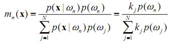
The KNN algorithm [8] assumes that pixels close to each other in feature space are likely to belong to the same class. It bypasses density function estimation and goes directly to a decision rule. Several decision rules have been developed, including a direct majority vote from the nearest k neighbours in the feature space among the training samples, a distance-weighted result and a Bayesian version [9]. If x is an unknown pixel vector and suppose there are kn neighbours labelled as class ωn out of k nearest neighbours,

(N is the number of classes defined). The basic KNN rule is

If the training data of each class is not in proportion to its respective population, p(ωn) in the image, a Bayesian Nearest-Neighbour rule is suggested based on Bayes’ theorem
 1 1
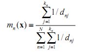
The basic rule does not take the distance of each neighbour to the current pixel vector into account and may lead to tied results every now and then. Weighted-distance rule is used to improve upon this as
 2 2
where dnj is Euclidean distance. With n training samples, one needs to find the k nearest neighbours for every pixel in a large image. This means n spectral distances must be evaluated for each pixel. The algorithm is summarised as below. The variable “unknown” denotes the number of pixels whose class is unknown and the variable “wrong” denotes the number of pixels which have been wrongly classified.
set number of pixels = 0
set unknown = 0
set wrong = 0
For all the pixels in the test image
do
{
1. Get the feature vector of the pixel and increment number of pixels by 1.
2. Among all the feature vectors in the training set, find the sample feature vector which is nearest (nearest neighbour) to the feature vector of the pixel.
3. If the number of nearest neighbours is more than 1, then check whether the corresponding class labels of all the nearest sample feature vectors are the same. If the corresponding class labels are not the same, then increment unknown by 1 and go to Step 1 to process the next pixel else go to Step 4.
4. Class label of the image pixel = class label of the nearest sample vector. Go to Step 1 to process the next pixel.
}
C. Neural network (NN)
NN classification overcomes the difficulties in conventional digital classification algorithms that use the spectral characteristics of the pixel in deciding the category of a pixel [7]. NN based Multi-Layer Perceptron (MLP) classification in RS use multiple layer feed-forward networks that are trained using the back-propagation algorithm based on a recursive learning procedure with a gradient descent search. A detailed introduction can be found in literatures [5 and 10].
There are numerous algorithms to train the network for image classification. A comparative performance of the training algorithms for image classification by NN is presented in Zhou and Yang, (2010) [11]. The MLP in this work is trained using the error backpropagation algorithm. The main aspects here are: (i) the order of presentation of training samples should be randomised from epoch to epoch; and (ii) the momentum and learning rate parameters are typically adjusted (and usually decreased) as the number of training iterations increases. Back propagation algorithm for training the MLP is briefly stated in Kumar et al. (2011) [7].
D. Random Forest (RF)
RF are ensemble methods using tree-type classifiers  where the where the are i.i.d. (independent and identically distributed) random vectors and are i.i.d. (independent and identically distributed) random vectors and  is the input pattern [12]. They are a combination of tree predictors such that each tree depends on the values of a random vector sampled independently and with the same distribution for all trees in the forest. It uses bagging to form an ensemble of classification tree [12]. RF is distinguished from other bagging approaches in that at each splitting node in the underlying classification tree, a random subset of the predictor variable is used as potential variable to define split. In training, it creates multiple CART (Classification and Regression Tree) trained on a bootstrapped sample of the original training data, and searches only across randomly selected subset of the input variables to determine a split for each node. It utilises Gini index of node impurity [13] to determine splits in the predictor variables. While classification, each tree casts a unit vote for the most popular class at input is the input pattern [12]. They are a combination of tree predictors such that each tree depends on the values of a random vector sampled independently and with the same distribution for all trees in the forest. It uses bagging to form an ensemble of classification tree [12]. RF is distinguished from other bagging approaches in that at each splitting node in the underlying classification tree, a random subset of the predictor variable is used as potential variable to define split. In training, it creates multiple CART (Classification and Regression Tree) trained on a bootstrapped sample of the original training data, and searches only across randomly selected subset of the input variables to determine a split for each node. It utilises Gini index of node impurity [13] to determine splits in the predictor variables. While classification, each tree casts a unit vote for the most popular class at input  . The output of the classifier is determined by a majority vote of the trees that result in the greatest classification accuracy. . The output of the classifier is determined by a majority vote of the trees that result in the greatest classification accuracy.
It is superior to many tree-based algorithms, because it lacks sensitivity to noise and does not overfit. The trees in RF are not pruned; therefore, the computational complexity is reduced. As a result, RF can handle high dimensional data, using a large number of trees in the ensemble. This combined with the fact that random selection of variables for a split seeks to minimise the correlation between the trees in the ensemble, results in error rates that have been compared to those of Adaboost, at the same time being much lighter in implementation. RF has also outperformed CART and similar boosting and bagging-based algorithm [14].
E. Contextual classification using sequential maximum a posteriori (SMAP) estimation
Spectral signatures are extracted from images based on training map by determining the parameters of a spectral class Gaussian mixture distribution model, which are used for subsequent segmentation (i.e. classification) of the multispectral (MS) images. The Gaussian mixture class describes the behaviour of an information class which contains pixels with a variety of distinct spectral characteristics. For example, forest, grasslands or urban areas are information classes that need to be separated in an image. However, each of these information classes may contain subclasses each with its own distinctive spectral characteristic; a forest may contain a variety of different tree species each with its own spectral behaviour. Mixture classes improve segmentation performance by modelling each information class as a probabilistic mixture with a variety of subclasses. In order to identify the subclasses, clustering is first performed to estimate both the number of distinct subclasses in each class, and the spectral mean and covariance for each subclass. The number of subclasses is estimated using Rissanen's minimum description length (MDL) criteria. This criteria determines the number of subclasses which best describe the data. The approximate Maximum Likelihood estimates of the mean and covariance of the subclasses are computed using the expectation maximization (EM) algorithm.
SMAP improves segmentation accuracy by segmenting the image into regions rather than segmenting each pixel separately [15]. The algorithm exploits the fact that nearby pixels in an image are likely to have the same class and segments the image at various scales or resolutions using the coarse scale segmentations to guide the finer scale segmentations. In addition to reducing the number of misclassifications, the algorithm generally produces segmentations with larger connected regions of a fixed class. The amount of smoothing that is performed in segmentation is dependent on the behaviour of the data. If the data suggest that the nearby pixels often change class, then the algorithm adaptively reduces the amount of smoothing, ensuring that excessively large regions are not formed (http://wgbis.ces.iisc.ac.in/grass/grass70/ manuals/html70_user/i.smap.html).
Support Vector Machine (SVM)
SVM are supervised learning algorithms based on statistical learning theory and heuristics [1 and 16]. SVM map input vectors to a higher dimensional space where a maximal separating hyper plane is constructed. Two parallel hyper planes are constructed on each side of the hyper plane that separates the data. The separating hyper plane maximises the distance between the two parallel hyper planes with an assumption that larger the margin between these parallel hyper planes, the better the generalisation error. The model produced by support vector classification only depends on a subset of the training data, because the cost function for building the model does not take into account training points that lie beyond the margin [1]. The success of SVM depends on the training process. The easiest way to train SVM is by using linearly separable classes.
Free and Open Source (FOS) Packages
The FOS Packages and model parameters to implement each algorithm (in Intel Pentium IV Desktop Computer, 3.00 GHz clock speed with 3.5 GB RAM and 1000 GB HD) are summarized next. For DT, rulesets were extracted using See5 (http://www.rulequest.com) with 25% global pruning. These rules were then used to classify Landsat ETM+ MS data. For KNN (algorithm was implemented in C programming language in Linux Platform), the number of nearest neighbour was kept 1 in feature space. In case of conflict, random allocation to LU class was done. NN based classification was implemented in C programming language, where a logistic function was used along with 4 hidden layer. Output activation threshold was set to 0.001, training momentum was set to 0.2, training RMS exit criteria was set to 0.1, training threshold contribution was 0.1, and the training rate was maintained at 0.2 to achieve the convergence. RF was implemented using a random forest package available in R interface (http://www.r-project.org). SMAP was implemented through free and open source GRASS GIS (http://wgbis.ces.iisc.ac.in/grass). SVM was implemented using both polynomial and RBF using libsvm package (http://www.csie.ntu.edu.tw/~cjlin/libsvm/). A second degree polynomial kernel was used with 1 as bias in kernel function, gamma as 0.25 (usually taken as 1 divided by the number of input bands), and penalty as 1. For RBF, gamma was 0.25 and penalty parameter was set to 1.
|
