| |
Indicators |
Formula |
Range |
Significance/ Description |
| Category : Patch area metrics |
| 1. |
Percentage of Landscape (PLAND) |
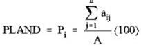
Pi = proportion of the landscape occupied by patch type (class) i.
aij = area (m2) of patch ij.
A = total landscape area (m2). |
0 < PLAND ≤ 100 |
PLAND is 0 when patch type (class) becomes increasingly rare in the landscape. PLAND = 100 with single patch type; |
| 2. |
Largest Patch Index(Percentage of landscape) |
aij = area (m2) of patch ij
A= total landscape area |
0 ≤ LPI≤100 |
LPI = 0 when largest patch of the patch type becomes increasingly smaller. LPI = 100 when the entire landscape consists of a single patch |
| 3. |
Number of Urban Patches |
 N N
NP equals the number of patches in the landscape. |
NPU>0, without limit. |
Higher the value more the fragmentation |
| 4. |
Patch
Density |
F (sample area) = (Patch Number/Area) * 1000000 |
PD>0,without limit |
Patch density increases with a greater number of patches within a reference area. |
| Category : Edge/border metrics |
| 5. |
Area weighted mean patch fractal dimension
(AWMPFD) |
Where si and pi are the area and perimeter of patch i, and N is the total number of patches |
1≤AWMPFD≤2 |
AWMPFD is 1 for shapes with very simple perimeters, such as circles or squares, and approaches 2 for shapes with highly convoluted perimeter |
| 6. |
Percentage of Like Adjacencies (PLADJ) |
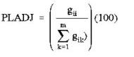
gii = number of like adjacencies (joins) between pixels of patch type (class) i based on the double-count method.
gik = number of adjacencies (joins) between pixels of patch types (classes) i and k based on the double-count method. |
0<=PLADJ<=100 |
The percentage of cell adjacencies involving the corresponding patch type that are like adjacencies. Cell adjacencies are tallied using the double-count method in which pixel order is preserved, at least for all internal adjacencies |
| 7. |
Mean Patch Fractal Dimension (MPFD) |
pij = perimeter of patch ij
aij= area weighted mean of patch ij
N = total number of patches in the landscape |
1<=MPFD<2 |
Shape Complexity.
MPFD approaches one for shapes with simple perimeters and approaches two when shapes are more complex. |
| Category : Shape metrics |
| 8. |
NLSI(Normalized Landscape Shape Index) |
Where si and pi are the area and perimeter of patch i, and N is the total number of patches. |
0≤NLSI<1 |
NLSI = 0 when the landscape consists of single square or maximally compact almost square and is 1 when the patch type is maximally disaggregated |
| Category: Compactness/ contagion / dispersion metrics |
| 9. |
Clumpiness |
gii =number of like adjacencies (joins) between pixels of patch type (class) I based on the double-count method.
gik =number of adjacencies (joins) between pixels of patch types (classes) i and k based on the double-count method.
min-ei =minimum perimeter (in number of cell surfaces) of patch type (class)i for a maximally clumped class.
Pi =proportion of the landscape occupied by patch type (class) i. |
-1≤ CLUMPY ≤1. |
It equals 0 when the patches are distributed randomly, and approaches 1 when the patch type is maximally aggregated |
| 10. |
Aggregation index |
max-gii = maximum number of like adjacencies (joins) between pixels of patch type class i based on single count method.
Pi= proportion of landscape comprised of patch type (class) i. |
1≤AI≤100 |
AI equals 1 when the patches are maximally disaggregated and equals 100 when the patches are maximally aggregated into a single compact patch. |
| 11. |
Interspersion and Juxtaposition |
eik = total length (m) of edge in landscape between patch types (classes) i and k.
E = total length (m) of edge in landscape, excluding background
m = number of patch types (classes) present in the landscape, including the landscape border. |
0≤ IJI ≤100 |
IJI is a measure of patch adjacency. IJI approach 0 when distribution of adjacencies among unique patch types becomes uneven; is equal to 100 when all patch types are equally adjacent to all other patch types. |
| 12. |
Cohesion |
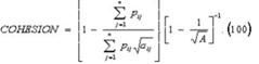 |
0≤cohesion<100 |
Patch cohesion index measures the physical connectedness of the corresponding patch type. |
| 13. |
Built up Area |
------ |
>0 |
Total built-up land (in ha) |
