|
RESULTS & DISCUSSION
Land use analysis: Land use analysis using Gaussian Maximum Likelihood Classifier was done for multi-resolution data (MODIS, Landsat, Ikonos and IRS P6) and the results are presented in Table 2 and figure 4. Overall accuracy of the classification was 88% using Landsat data, 91% accuracy using IRS-P6 data and 74% using Modis data respectively.
Table 2. Land use details of the study region
| Class |
Urban |
Vegetation |
Water |
Others |
| Res. |
Ha |
% |
Ha |
% |
Ha |
% |
Ha |
% |
| 500 |
1677.2 |
95.5 |
--- |
--- |
--- |
--- |
59.9 |
3.45 |
| 30 |
1034.8 |
59.0 |
390.1 |
22.2 |
2.7 |
0.1 |
325.4 |
18.5 |
| 5 |
1125.7 |
64.2 |
370.7 |
21.1 |
3.0 |
0.1 |
253.9 |
14.4 |
| 4 |
1145.3 |
65.3 |
350.7 |
20.0 |
3.0 |
0.1 |
254.2 |
14.5 |
Note: Res.: Spatial resolution (in m)
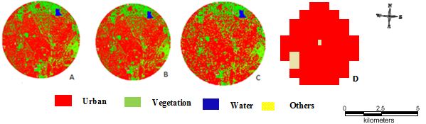
Figure 2: Land use statistics A). Ikonos 4m b). IRS-P6 5 m c). Landsat-30m d). Modis-500m
Landscape Metrics: Landscape metrics were computed for varied resolution of multi resolution data for sample space in Greater Bangalore. The data was classified into 4 land use categories in a heterogeneous landscape, Urban category was considered for further analysis as the landscape is rapidly urbanizing and constitute a dominant class. Table 3. lists the quantified values of each metrics across resolutions of multi-resolution data.
Table 3: Spatial metrics computed for classified multi resolution data using FRAGSTAT
| Resolution |
NP |
LPI |
NLSI |
| 500, MODIS |
1 |
38.88 |
0.051 |
| 250, MODIS |
1 |
34.98 |
0.045 |
| 100, MODIS |
1 |
35.98 |
0.054 |
| 30, LANDSAT |
12 |
31.74 |
0.056 |
| 15, LANDSAT |
254 |
38.08 |
0.028 |
| 5, IRS P6 |
1566 |
34.39 |
0.091 |
| 4, IKONOS |
1571 |
47.82 |
0.094 |
| 3, IKONOS |
2193 |
72.76 |
0.045 |
| 2, IKONOS |
2480 |
84.36 |
0.024 |
| Resolution |
CLUMPY |
PLADJ |
IJI |
| 500, MODIS |
0.915 |
82.143 |
-------------- |
| 250, MODIS |
0.973 |
89.49 |
------------ |
| 100, MODIS |
0.973 |
89.50 |
----------- |
| 30, LANDSAT |
0.917 |
93.66 |
52.48 |
| 15, LANDSAT |
0.945 |
92.78 |
52.35 |
| 5, IRS P6 |
0.857 |
90.76 |
65.71 |
| 4, IKONOS |
0.854 |
90.49 |
96.65 |
| 3, IKONOS |
0.862 |
92.36 |
96.65 |
| 2, IKONOS |
0.862 |
96.35 |
96.65 |
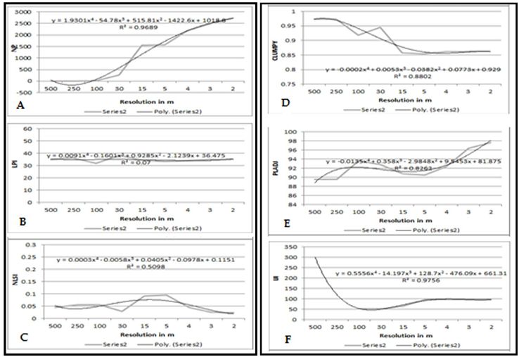
Figure 4: Correlation of spatial matrices with varied resolutions of the data
Number of Patches (NP) tabulated in table 3, indicates the level of fragmentation. The results highlight the indices dependence on spatial resolutions evident from the refinement of values with finer spatial resolutions. Number of Patches (NP) indicates that smaller patches aggregating to form a cluster of the urban surface. Figure 4a. indicate that better spatial resolution reveals large number of smaller patches and as the resolution becomes finer the number of patches becomes precise.
Largest patch index (LPI) indicates that the landscape is in the process of aggregation to be a single patch, indicating homogenisation of landscape. This metrics is not dependent on resolutions as it quantifies the largest patch and almost accurately in all resolutions as illustrated in Figure 4b.
Clumpiness index, Interspersion and Juxtaposition Index (IJI) highlights the occurrence of same patch in the neighborhood. Clumpiness index mainly highlight the nature of development of a particular class with the neighborhood. If the value of IJI is not obtained it means to say that the patch types distinctly pound is less than three. All resolution output for all these metrics indicates that higher or better resolution is necessary to obtain appropriate result. Figure 4d and 4f corresponding to these spatial metrics indicates of improvements with the finer spatial resolutions.
Percentage of like adjacency (PLADJ) indicates the frequency of different pairs of patch types occurring, measuring the degree of aggregation of the focal patch type. The values close to 0 indicates maximally dispersed pattern and values close to 100 indicates maximally contagious. Figure 4e highlight the dependence on spatial resolutions as lower resolution images fails to give an appropriate result.
Normalized Landscape Shape Index (NLSI) indicates the shape of the landscape. Values close to 0 indicates that the landscape under study has simple shape means to say it is further aggregating to become a single patch. Values close to 1 indicates that the landscape has a complex shape. Figure 4c highlight that the regions are becoming a single patch of the simple size and independent of resolutions.
|
