Commuting CO2 emission distribution, model results, and countermeasure analysis

5.1 Key challenges revealed from distribution of commuting CO2 emissions

The percentiles of the individuals and households commuting CO2 emissions in Xi’an and Bangalore are shown in Fig. 2. It is seen that the emissions in Xi’an are lower than those in Bangalore except the highest 10 % households. The average and median values of the individual and household emissions in Table 7 also show that the emissions in Bangalore are higher than those in Xi’an. The average individual CO2 emissions by modes in Table 7 and emission factor by modes in Table 3 indicate that longer commuting distance is a major factor for higher CO2 emissions in Bangalore. The average commuting distance in Bangalore (7.09 km) is twice of that in Xi’an (3.8 km). The longer distance in Bangalore is due to its haphazard and dispersed urban growth, and the shorter distances in Xi’an can be attributed to its compact and high-density pattern. Thus, one key challenge for Indian cities is to develop the compact and high-density urban pattern so as to reduce their commuting distances and improve their public transit operation efficiency.

It is found that, in Xi’an, 20 % of the commuters produced 78 % the total emissions; in Bangalore, 20 % of the commuters produced 56 % the total emissions. Also, 20 % of the households produced 73 % the total emissions in Xi’an; 20 % of the households produced 53 % the total emissions in Bangalore. Therefore, generally, B70-20^ and B50-20^ emission patterns exist in Xi’an and Bangalore, respectively. This result is different from the B60-20^ emission rule in UK (Brand and Preston 2010; Susilo and Stead 2009), the B50-10^ emission rule in Dutch (Susilo and Stead 2009), and the B60-10^ emission rule in Seoul (Ko et al. 2011), which indicates that the high emitters produce a disproportionate fraction of the total emissions. It also indicates that the high emitters produced higher proportion of CO2 emissions in Chinese cities. Thus, another key challenge for Chinese and Indian cities, especially for Chinese cities, lies in that they should focus on reducing CO2 emissions from the high emitters. Other global cities’ experiences of reducing the transportation CO2 emissions may also be applied to Indian cities.

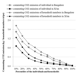
Figure 2 Commuting CO2 Emissions by percentiles in Xi’an and Bangalore

Table 7 Summary of commuting CO2 emissions, population, and vehicles in Xi’an and Bangalore

^aIn Bangalore, the average commuting CO2 emissions by car include both car and two-wheelers
^bThe data refers to the population in the Xi’an urban central area
^c In Bangalore, LMV refers to the light motor vehicle

^dIn Xi’an, there is prohibition of two-wheelers inside the 2nd Ring Road

Figures 3 and 4 present the spatial distributions of household and individual commuting CO2 emissions in Xi’an and Bangalore, respectively. It is seen that Bangalore has higher emissions than Xi’an in general, and households and individuals located in the outer areas produce much more emissions than those in the inner areas and CBDs. The highest emissions scattered along/outside the 2nd Ring Road in Xi’an and the Outer Ring Road in Bangalore, respectively. These indicate that, from the urban spatial perspective, the key challenge of low-carbon development is to reduce higher emissions along the ring roads and in the outer areas.

5.2 Tobit models for CO2 emissions by commuters and corresponding countermeasures

5.2.1 Tobit model results

The Tobit models for commuting CO2 emissions are shown in Table 8 below. The results show that the car availability is the key factor of both household and individual commuting CO2 emissions in the two cities. The coefficients of the car availability in Xi’an models are bigger

Fig. 3 Distributions of average household commuting CO2 emissions by zone (kg/household, sum of commut-ing CO2 emissions of each commuter in the household)

than those in the corresponding Bangalore models. This is because there are more cars in Xi’an than in Bangalore and because the two wheelers account for 77.1 % of the car and two-wheeler in Bangalore. It is the first time that our method found that household locations separated by the ring roads have a great impact on both household and individual commuting CO2 emissions in all the four models. Households and individuals located outside the 2nd or

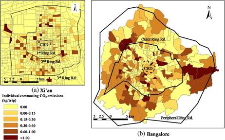
Fig. 4 Distributions of average individual commuting CO2 emission by zone (kg/trip)

Table 8 Tobit models for commuting CO2 emissions
                                                                 

The numbers in the brackets refer to significance levels. In Bangalore, car availability includes both cars and two-wheelers. In Xi’an, car availability refers to people owning car or willing to buy car

Outer Ring Road produced larger CO2 emissions than those located in the inner areas. This indicates that geographic location separated by the ring roads is a good indicator of the commuting CO2 emissions. It is related to mode supply, mixed level of land use, and the commuting distances in the areas separated by the ring roads, and it has great values in the urban planning and management practice. The average commuting distance is 5.51 km inside the CBD of Bangalore and increases sharply to 7.32 km outside the CBD and to 8.44 km outside the Outer Ring Road. The average commuting distance is 2.88 km inside the 1st Ring Road of Xi’an and increases to 3.22, 4.03, and 5.09 km between the 1st and 2nd Ring Roads, between the 2nd and 3rd Ring Roads, and outside the 3rd Ring Road, respectively, as shown in Fig. 5a. By analyzing Figs. 3, 4, and 5a, we can find that there are longer average commuting distance, higher average and total commuting CO2 emissions, and more average emission distributions among the individuals and households in Bangalore than in Xi’an. Considering the future rapid economic growth, urbanization, and motorization in Bangalore, there is a need to reduce the possible sharp increase of the commuting CO2 emissions in Indian cities. In addition, the percentages of the car availability in different household locations separated by the ring roads are also different. There is a higher percentage of car availability in the outer area

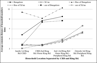
(a) Average commute distance of household members by household locationand by travel mode

(b) average commute distance of household members by household locationand by travel mode
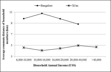
Average commute distance of household members by household annual income

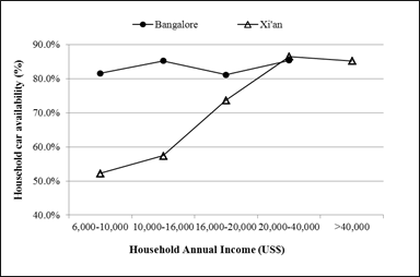
(c)Percentage of household car availability by household annual income

(d) Average commute distance of household members by household locationand by travel mode

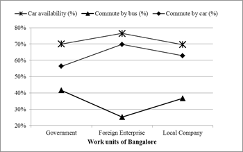
(e) Car availability and car/bus shares by work unit type in Bangalore

than that in the inner area. According to the statistical results, in Xi’an, the percentages of car availability are 36.8, 52.4, and 61.6 %, respectively, for the sampled households inside the 1st Ring Road, between the 1st and 2nd Ring Roads, and between the 2nd and 3rd Ring Roads. In Bangalore, the percentages of sampled households with car availability between the CBD and Outer Ring Roads and between the Outer and Peripheral Ring Roads are 71.5 and 73.2 %, respectively.

Apart from the household location separated by the ring roads and car availability, household annual incomes have been proven to be another key factor of the household commuting CO2 emissions in Xi’an and Bangalore. The result of Xi’an model shows that household commuting CO2 emissions increase with the household annual income’s increase. It could be because the households with higher income tend to have longer commuting distance and higher percentage of car availability. Details are shown in Fig. 4b, c. The impact of household annual income on the household CO2 emission in Bangalore model is different from that in Xi’an model. It is found that, in Bangalore model, household commuting CO2 emissions are not linearly increasing with the household annual income’s increase as in Xi’an model. Also, the households with middle-level income of US$ 10,000–16,000 tend to produce the highest commuting CO2 emissions; correspondingly, these households have the longest commuting distances and the highest percentage of the car and two-wheeler’s availability, as shown in Fig. 4b, c.

Previous studies found that full-time workers produced more transportation CO2 emissions than part-time workers (Carlsson-Kanyama and Lindén 1999; Susilo and Stead 2009; Ko et al. 2011; Brand et al. 2013) and unemployed (Brand and Boardman 2008). While in this study, for the first time, we found that the type of work unit for the full-time worker is a key factor for the commuting CO2 emissions in Bangalore’s model, even though this factor is not significant in the Xi’an model. In Bangalore, foreign company workers produce higher CO2 emissions than the government staff and the workers in local and state-owned companies. This is mainly due to the long commuting distance, high percentages of the car and two-wheeler’s availability, and the high percentage of car uses among the foreign company workers, as shown in Fig. 4d, e. In addition, this is also because the household annual income of foreign company workers in Bangalore is 22 % higher than the overall average level.

Distance to the nearest bus stop is another factor of the individual commuting CO2 emissions in Bangalore. The model results show that 0.107 kg more individual CO2 emissions can be produced if the commuters live 1 km farther away from the nearest bus stop. However, in Xi’an models, this factor is not significant.

In summary, there are two common factors which affected the commuting CO2 emissions in the all models of Xi’an and Bangalore, car availability and household location separated by the ring roads. For household CO2 emission models of Xi’an and Bangalore, household annual income is a significant factor. The difference between the models lies in that work unit type and distance to the nearest bus stop are only significant in Bangalore’s individual emission model.

5.2.2 Countermeasures based on the model results

The results of the Tobit models show that the positive factors for the commuting CO2 emissions in Bangalore include car availability, high household income, working in foreign company, living in the outer areas of city, and distance to the nearest bus stop. The positive factors for the commuting CO2 emissions in Xi’an include car availability, high household income, and living in the outer areas of city. Among these factors, car availability has the

largest impact on the commuting CO2 emissions, followed by household income, working in foreign company, living in the outer areas, and distance to the nearest bus stop. Consequently, the key countermeasure to reduce the high CO2 emissions is to encourage the emitters to take public transit instead of driving cars. As there is a high requirement on the comfort and convenience for trips by high emitters, the high emitters will not use public transit if the bus service is poor or the bus is inconvenient. Therefore, only by providing good public transit service and high bus stop coverage rate, mixed with the car demand management policy at the same time, the high emitters with car availability can take public transit.

In Xi’an and Bangalore, the closer to the city center, the higher the population density is and the severer the traffic congestions are. In contrary, the farther to the city center, the better the road conditions are and the higher the car availability is. Since the public transit typically costs passengers more travel time than self-driving, the residents with car availability, far away from the bus stop, and living in the outer areas or along the ring roads are more likely to commute by driving. As the city sprawls, the commuting distance of the residents living in the outer area of the city will be longer and longer. Consequently, the traffic congestion will be easily formed in a large scale with commuting CO2 emissions increasing sharply in the central urban area. Therefore, there is a need to develop rapid transit system from the outer area to the inner area in the cities of China and India, such as rail transit and bus rapid transit (BRT). Due to the reason that there is no link between the land development revenue and the transportation investment in the early stage of urban development in both Xi’an and Bangalore, metro- or BRT-oriented development is hard to be implemented now. In other words, fund shortage for the transit-oriented development (TOD) in new developing areas in the early stage of urban development can further cause the shortage of the land for public transit terminal, transfer, and facilities and finally leads to the high commuting CO2 emissions. In addition, it is necessary to implement parking demand control in the industrial development area, especially in the area with foreign companies and government in Indian cities; at the same time, the good transit service should be developed.