Results and Discussion |
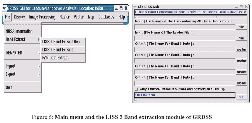
The SOI toposheets (scale 1: 50,000 and 1:250,000) were digitized using GRASS 5.0.0. Separate base layers were created for boundary, road network, drainage network, forest land, built up land, and water bodies. The multispectral LISS-III satellite imagery procured from NRSA, Hyderabad, India was extracted using the band extraction module of GRDSS, which is given in figure 6.
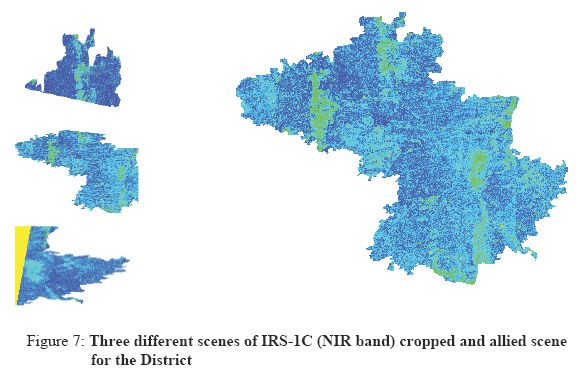
The respective band images were rectified using nearest neighbour resampling algorithm (geometric correction) considering field data collected (ground control points) using GPS and by vector layer obtained by digitization of toposheets. When mutually identified on the ground and on a satellite image, GCPs (Ground control points) were marked precisely to establish the exact spatial position and orientation of the satellite imagery relative to the ground at that instance. (Dwivedi et al., 2000). A new MAPSET and LOCATION was created in GRDSS database. The latitude-longitude coordinate system and the polyconic projection were assigned, and the images were transformed by the first order polynomial transformation. The respective band images corresponding to the district were cropped from the scenes. For this purpose, vector layer of district boundary was rasterised and each cell was assigned with a value of 1 for the region within the boundary and 0 elsewhere. Multiplication of this layer with the scene (100-63, 100-64 and 101-64) crops the information for the district. These scenes were allied to obtain the entire scene for the district as depicted in figure 7.
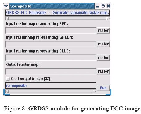
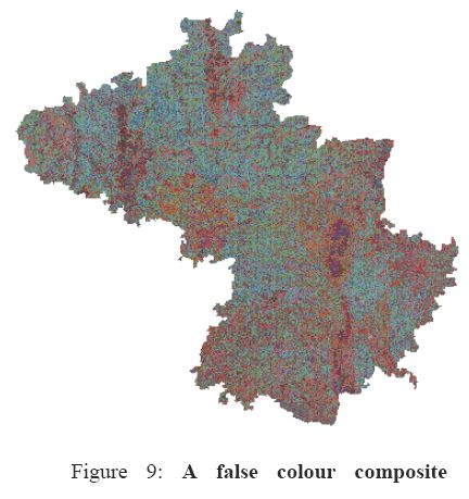
FCC was generated with the help of the composite module of GRDSS (given in Figure 8) using MSS data corresponding to band-2 (green), band-3 (red) and band-4 (near infrared) with a spatial resolution of 23.5 m. FCC helps in selection of training sites. Chosen training sites were uniformly distributed all over the district image covering all heterogeneous patches. The overall objective of the training process is to assemble a set of statistics that describe the spectral response pattern for each land cover type to be classified in an image. Attribute information corresponding to these heterogeneous patches was collected in the field using GPS.
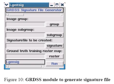
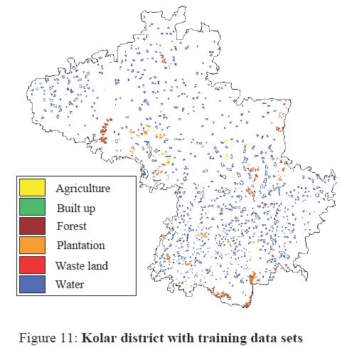
The vector layer of field data (figure 11) is rasterised and overlaid on MSS data to obtain the spectral signatures corresponding to the training sites. With this information, image was classified for major land use categories.
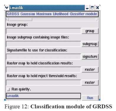
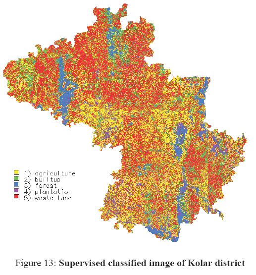
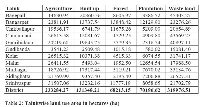
Supervised classification using Gaussian maximum likelihood classifier (GMLC) of the remote sensing data was done to classify the data in to categories - agriculture, forest, plantation, built-up and waste land and the classified image for the district is depicted in figure 13. Further, by overlaying taluk boundaries, taluk wise land use data was extracted. Talukwise landuse details as per supervised classification are listed in table 2. The data for March month was used for the analysis that corresponds to dry season, hence in the classified image there are no traces of water bodies.
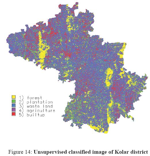
Unsupervised classification of the data was done to assess the relative merits of the two techniques namely supervised versus unsupervised. The histogram of the image was generated for deciding the initial number of classes and for choosing the number of clusters. The clustering algorithm was used and the image was classified into five categories using GMLC as shown in figure 14.
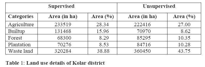
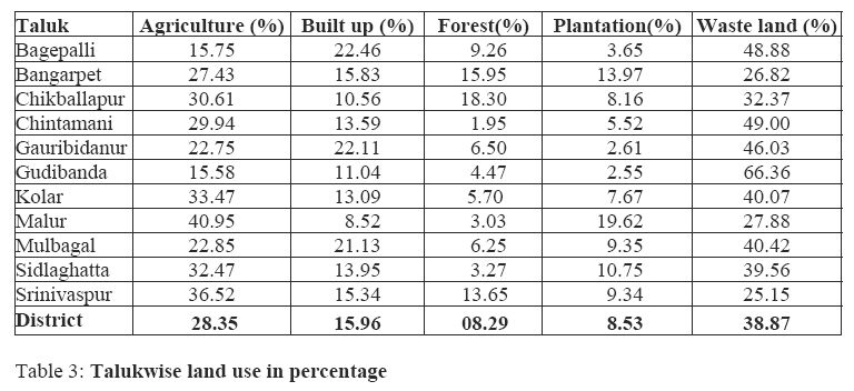
Composition of land use (in hectares) for Kolar as per supervised and unsupervised classification is given in table 1. Talukwise land use analyses details (in percentages) are listed in table 3.