2. Materials and methods

2.1 Study area

The study area, Kolar is located in Karnataka state, India. It lies in the plain regions (semi arid agro-climatic zone) extending over an area of 8238 sq. km. between 77°21’ to 78°35’ E and 12°46’ to 13°58’ N (shown in figure 2). For administrative purposes, it is divided into 11 taluks (or administrative boundaries /blocks/units). The distribution of rainfall is during southwest and northeast monsoon seasons. The average population density of the district is about 2.09 persons/hectare. The district forms part of northern extremity of the Bangalore plateau. The area is often subjected to recurring drought. The rainfall is both scanty and erratic in nature. The district is devoid of significant perennial surface water resources leading to limited ground water potential. The terrain has a high runoff due to less vegetation cover contributing to erosion of top productive soil layer leading to poor crop yield. Out of about 280 thousand hectares of land under cultivation, 35% is under well and tank irrigation (Ramachandra et al., 2005).

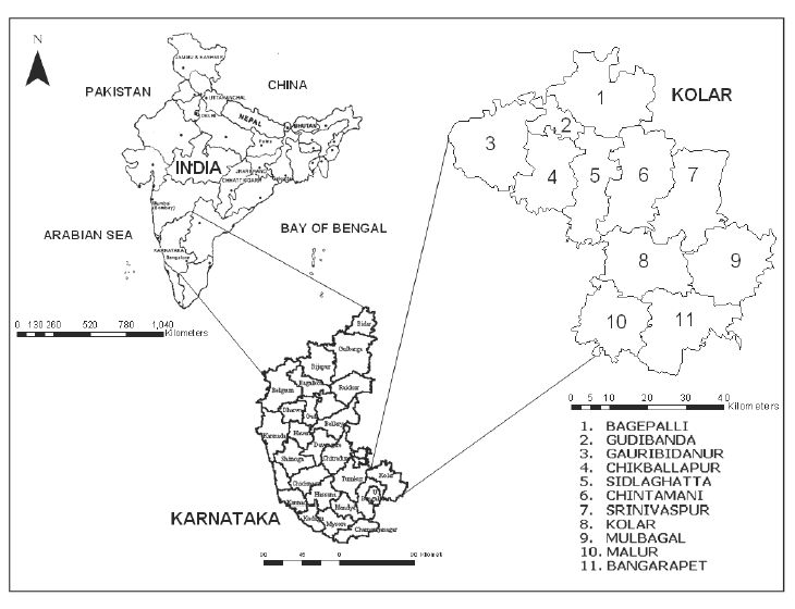
Figure 2: Study area – Kolar district, Karnataka State, India.

2.2 Data

MODIS data were downloaded from the Earth Observing System Data Gateway (http://edcimswww.cr.usgs.gov/pub/imswelcome/). These data sets are known as “MOD 09 Surface Reflectance 8-day L3 global” product with spatial resolutions 250 m (band 1 and band 2) and 500 m (band 1 to band 7). The MODIS Surface-Reflectance Product (MOD 09) is computed from the MODIS Level 1B land bands 1, 2, 3, 4, 5, 6, and 7 (centered at 648 nm, 858 nm, 470 nm, 555 nm, 1240 nm, 1640 nm, and 2130 nm, respectively). The product is an estimate of the surface spectral reflectance for each band as it would have been measured at ground level if there were no atmospheric scattering or absorption (http://modis.gsfc.nasa.gov/data/dataprod/dataproducts.php? MOD_NUMBER=09). Each MODIS Level-1B data product (Guenther et al., 1998), contains the radiometrically corrected, fully calibrated and geolocated radiances at-aperture for all 36 MODIS spectral bands at 1 km resolution (http://daac.gsfc.nasa.gov/MODIS/Aqua/product_descriptions_modis.shtml#rad_geo). These data are broken into granules approximately 5-min long and stored in Hierarchical Data Format (HDF). Bands 1 to 36 MODIS data “MOD 02 Level-1B Calibrated Geolocation, Data Set” were downloaded from EOS Data Gateway (http://edcimswww.cr.usgs.gov/pub/imswelcome/). The Level 1B data set contains calibrated and geolocated at-aperture radiances for 36 bands generated from MODIS Level 1A sensor counts (MOD 01). The radiances are in W/(m2 µm sr). In addition, Earth BRDF may be determined for the solar reflective bands (1-19, 26) through knowledge of the solar irradiance (e.g., determined from MODIS solar-diffuser data and from the target-illumination geometry). Additional data are provided, including quality flags, error estimates, and calibration data (http://modis.gsfc.nasa.gov/data/dataprod/ dataproducts.php? MOD_NUMBER=02). The Indian Remote Sensing (IRS) Satellites-1C/1D LISS 3 (Linear Imaging Self-Scanning Sensor 3) MSS (Multi Spectral Scanner) having 3 bands (G, R and NIR) data with a spatial resolution 23.5 m were procured from NRSA, Hyderabad. The main sources of primary data are from field (using GPS), the Survey of India (SOI) toposheets of 1:50,000, 1:250,000 scale and the secondary data were collected from the government agencies (Directorate of census operations, Agriculture department, Forest department and Horticulture department) etc.

2.3 Methods

The methods adopted in the analysis involved :

Creation of base layers like district boundary, district with taluk and village boundaries, road network, drainage network, mapping of water bodies, etc. from the SOI toposheets of scale 1:250000 and 1:50000.
Identification of ground control points (GCP’s) and geo-correction of MODIS (MOD 09 Surface Reflectance 8-day L3 global Products) band 1 and 2 (spatial resolution 250 m) and bands 3 to 7 (spatial resolution 500 m) and MOD 02 Level-1B Calibrated Geolocation Data Set band 1 to band 36 (spatial resolution 1 km).
Resampling of MODIS bands 3 to 7 (MOD 09 product) and MODIS bands 1 to 36 (MOD 02 product) to 250 m using nearest neighbourhood technique for easy processing, overlaying and comparison for analysis consistency.
Reprojection from Sinusoidal projection to Polyconic projection with Evrst 1956 as the datum, followed by masking of the study area.
Principal Component Analysis (PCA) of the MODIS 36 bands and derivation of Principal Components.
Derivation of Minimum Noise Fraction (MNF) of the MODIS 36 bands. It helped in to determine the inherent dimensionality of the data, to reduce noise and computational requirements for subsequent processing.
Classification of MODIS data using SAM and GMLC.
Extraction of high resolution LISS-3 bands from NRSA dataset (which were in BIL format), identification of ground control points (GCP’s) and geo-correction of the bands through resampling followed by cropping and mosaicing of data corresponding to the study area.
Generation of FCC (False Colour Composite) and identification of training sites (heterogeneous patches) on FCC. Heterogeneous patches correspond to various land features. Training sites are chosen so as to represent all land categories and uniformly spread all over the study area.
Collection of attribute information from field corresponding to the chosen training sites using GPS.
The training polygons collected from the field were overlaid on the FCC of the image and a region of interest (ROI) was created, thus enabling direct selection of assumed pure pixels (endmembers)
12 Scatter plots of bands helped in locating some of the purest endmembers by taking the extreme corner pixels. Finally, these spectra obtained by different methods (ROI and scatter plots) were merged into six classes.
Supervised Classification of LISS-3 MSS data using GMLC.
Accuracy Assessment of LISS-3 MSS classified data.
Accuracy assessment of MODIS classified data (using SAM and GMLC) and comparison with MSS classified data (pixel by pixel).