3. Results and Discussion |
Class spectral characteristics plot for the six classes across the first seven bands, PCs and MNF components of the 36 bands showed distinct pattern for respective categories. The similar pattern was observed in the Transformed Divergence matrices.The MODIS data were classified using the SAM technique. At an angle of 0.5 radians, the classified output of the MODIS bands 1 to 7 represented the 6 land cover classes. The first five PCs were then classified using SAM (the spectral angle set for classes are: 5 for agriculture, 5 for built up, 0.05 for forest, 0.02 for plantation, 3 for forest and 0.02 for water bodies) after iterations of tuning the angle between the class spectra and the reference spectra to avoid misclassifications. The five MNF components were also classified using the SAM. At an angle of 5 radians, all the classes represented the land cover classes well (except water, which was classified at an angle of 0.2 radians). The classified maps obtained using SAM are as shown in figure 3 (C), (D), and 4 (A).
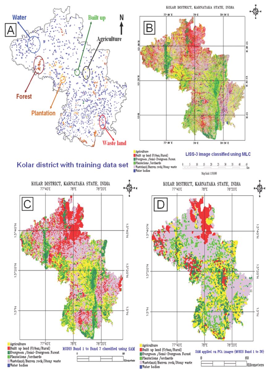
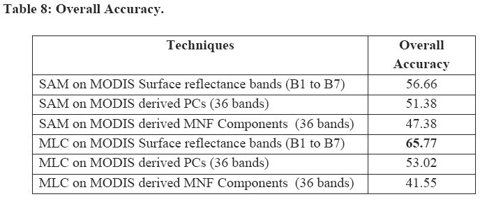
Figure 3: (A) Distribution of training data set over the district (B) MLC on LISS-3
MSS
(C) SAM on MODIS bands 1 to 7 (D) SAM on PCs.
FCC was created using MODIS bands 4 (Green), 1 (Red) and 2 (NIR). The heterogeneous patches were identified in the FCC as training regions for attribute data collection.
MODIS bands 1 to 7 were classified by Gaussian Maximum Likelihood Classifier (GMLC). At a threshold of 0.001, these 7 bands gave a good representation of the land cover classes. Similarly, Principal Components (PCs) of 36 bands were classified by GMLC maintaining a threshold of 0.001. The pixels in the MNF components were not very distinct and were clustered into sub groups (comprising of two or three pixels). Though, the class separation was possible, yet it was difficult to classify each pixel based on signature, since the image was slightly pixelated. The MNF components were also classified at a threshold of 0.001 as shown in figure 4 (B), (C) and (D).
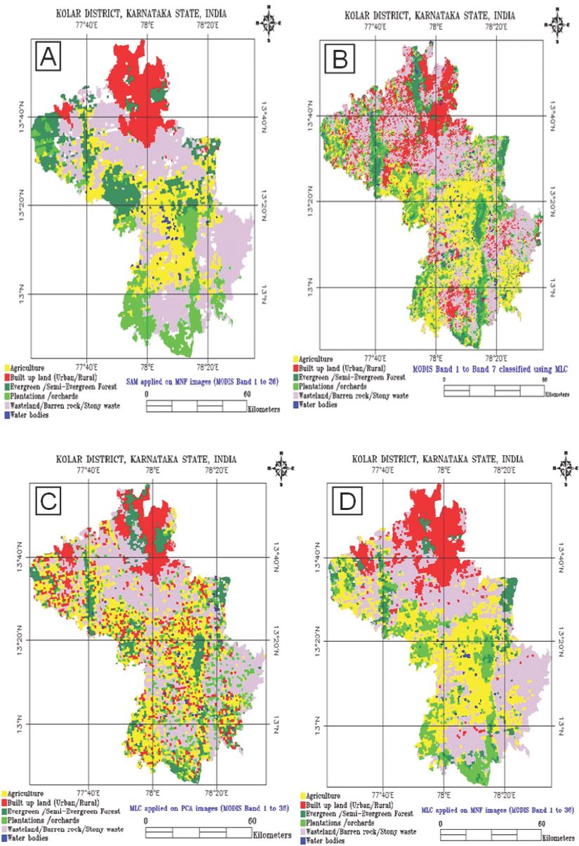
Figure 4: (A) SAM on MNF components (B) MLC on MODIS bands 1 to 7
(C) MLC
on PCs (D) MLC on MNF components.
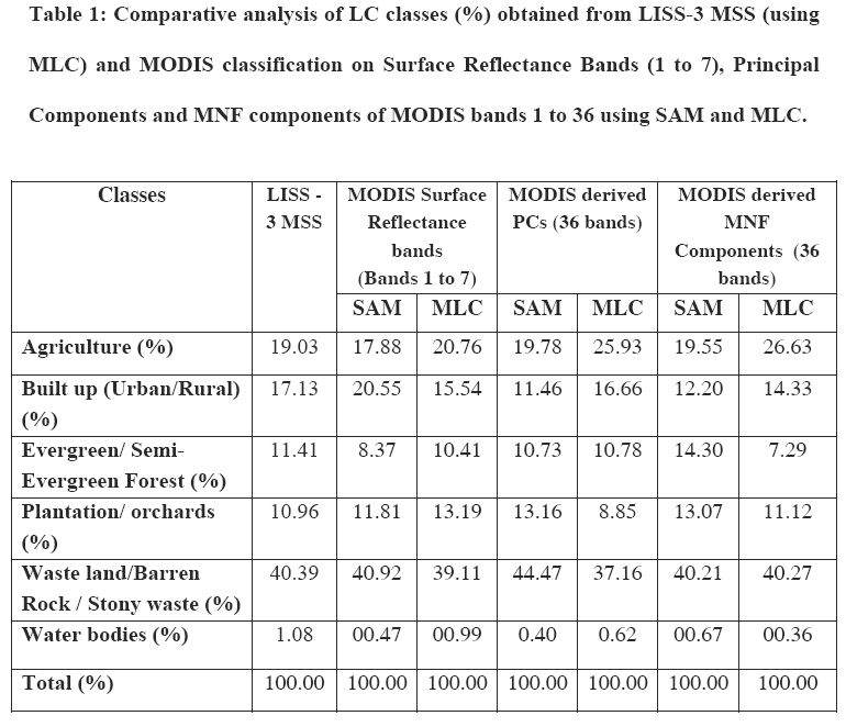
The class spectral characteristics for the six land cover classes considering LISS-3 MSS bands 2, 3 and 4 were generated to see separability among classes. The Transformed Divergence Matrix also helped in distinguishing different classes. False colour composite (FCC) was generated from the LISS-3 MSS data. The heterogeneous patches (training polygons) were chosen for the field data collection. This data with other ancillary data were used for classifying LISS-3 MSS data using GMLC. Care was taken to see that these training sets are uniformly distributed representing / covering the study area as shown in figure 3 (A). The supervised classified image shown in figure 3 (B) was validated by field visit and by overlaying the training sets used for classification. The land cover statistics are listed in table 1. Classified LISS-3 data aided as a reference high resolution image (with a spatial resolution of 23.5 m). Table 1 provides a comparative statistics of land cover using MODIS and LISS data with different classification approaches.
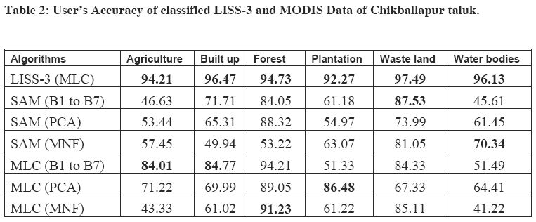
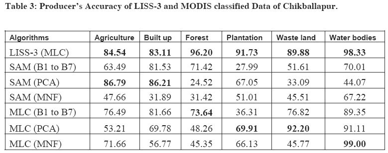
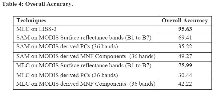
The accuracy assessment was done by collecting field data for Chikballapur taluk (which constitutes 10% of the study area Kolar district). The producers, users accuracy and overall accuracy corresponding to the various categories were computed, along with the error matrices for supervised classified MSS data of LISS-3, which is summarised in table 2, 3 and 4. The LISS-3 supervised classification accuracy assessment gave a kappa (k) value of 0.95 indicating that an observed classification is in agreement to the order of 95 percent.
Accuracy assessments of classified data were done 1) using field data, 2) comparing land cover percentage area for different taluks across various techniques and data, and 3) pixel to pixel comparison with the classified LISS-3 data.
Users, Producers and Overall accuracy assessment of the MODIS classified maps were done with the field data and the results are listed in tables 2, 3 and 4 respectively. Accuracy Assessment of MODIS classified maps were also performed at two spatial scales at the administrative boundary level (taluk) and at the pixel level.
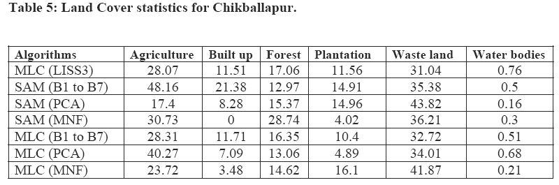
Land cover statistics were computed for all taluks pertaining to each classification algorithm and is given in table 5. The analysis showed that MLC on MODIS band 1 to 7 was better than all other techniques for mapping agriculture followed by SAM on MNF components whereas SAM on MODIS B1 to B7 performed poorly on this class. MLC on MODIS band 1 to 7 is also good for mapping built up areas, forest, plantation and waste land. On the other hand, MLC on PCs was good for mapping water bodies.
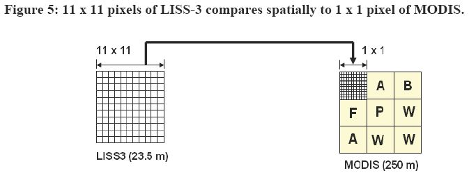
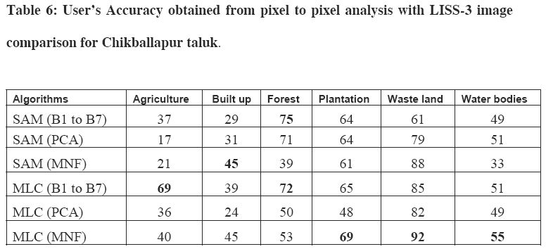
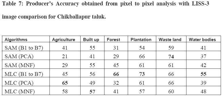
Classified data of MODIS and LISS-3 MSS were compared on a pixel by pixel basis for accuracy assessment of pure (homogenous) pixels. One pixel of MODIS spatially corresponds to 121 pixels (that is approximately equal to 258.5 m) of LISS-3 (figure 5). The error matrix was generated with users accuracy, producers accuracy and overall accuracy for the taluk and is listed in table 6, 7 and 8.
Further, within the land cover parameter, errors are generated either due to commission or omission when the signal of a pixel is ambiguous, perhaps as a result of spectral mixing, or when the signal is produced by a cover type that is not accounted for in the training process. With respect to a particular class, errors of omission occur when pixels of that class are assigned wrong labels; errors of commission occur when other pixels are wrongly assigned the label of the class considered. These errors are a normal part of the classification process, which can be minimized.